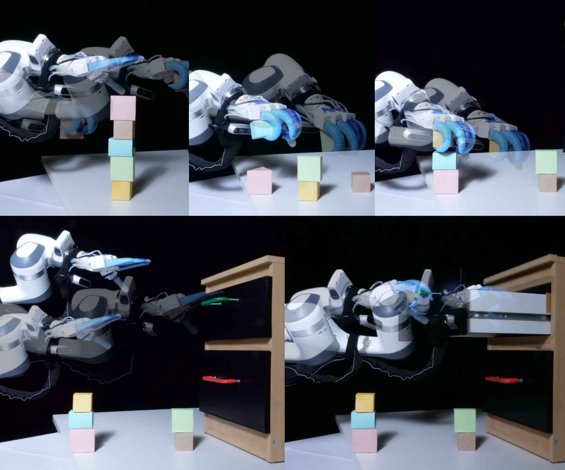
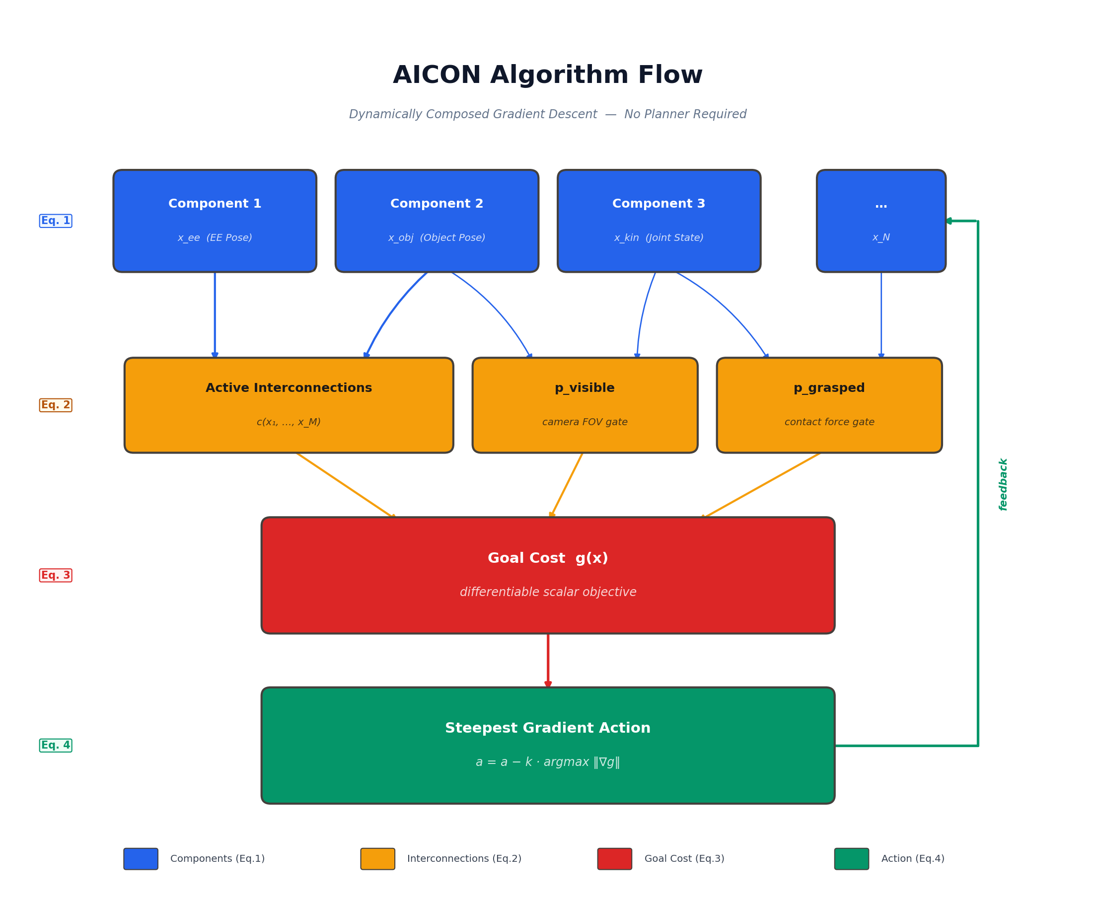
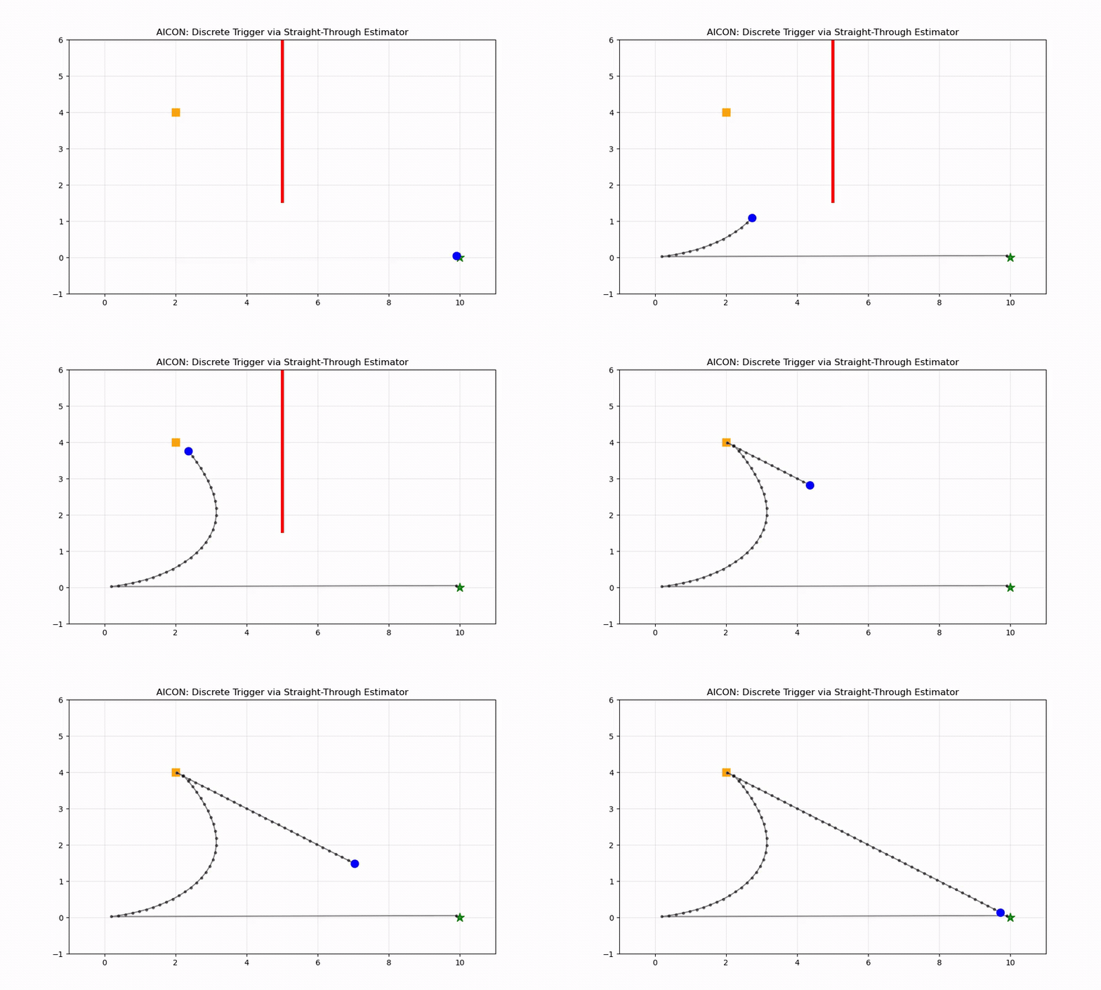
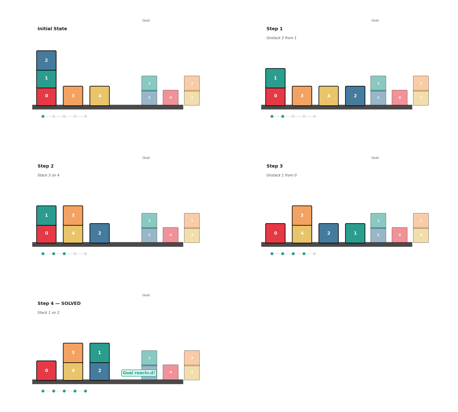
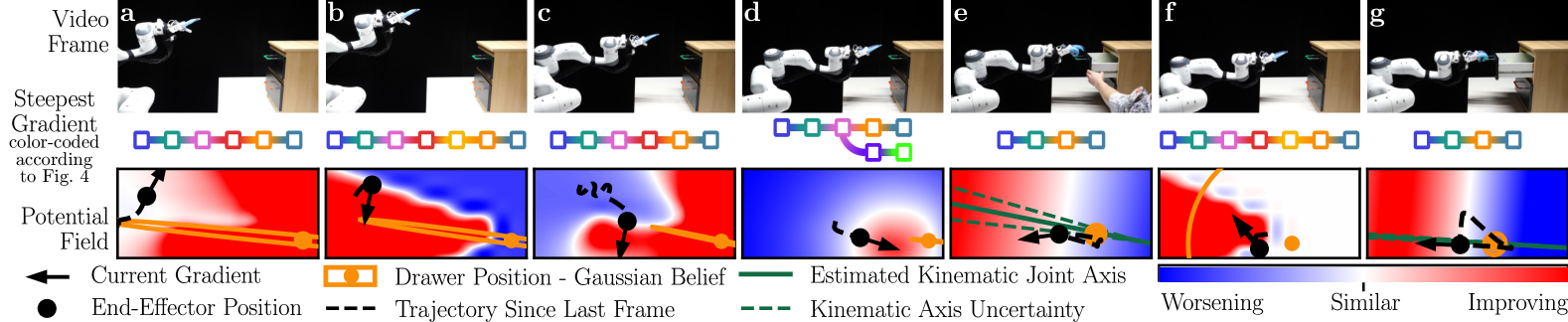
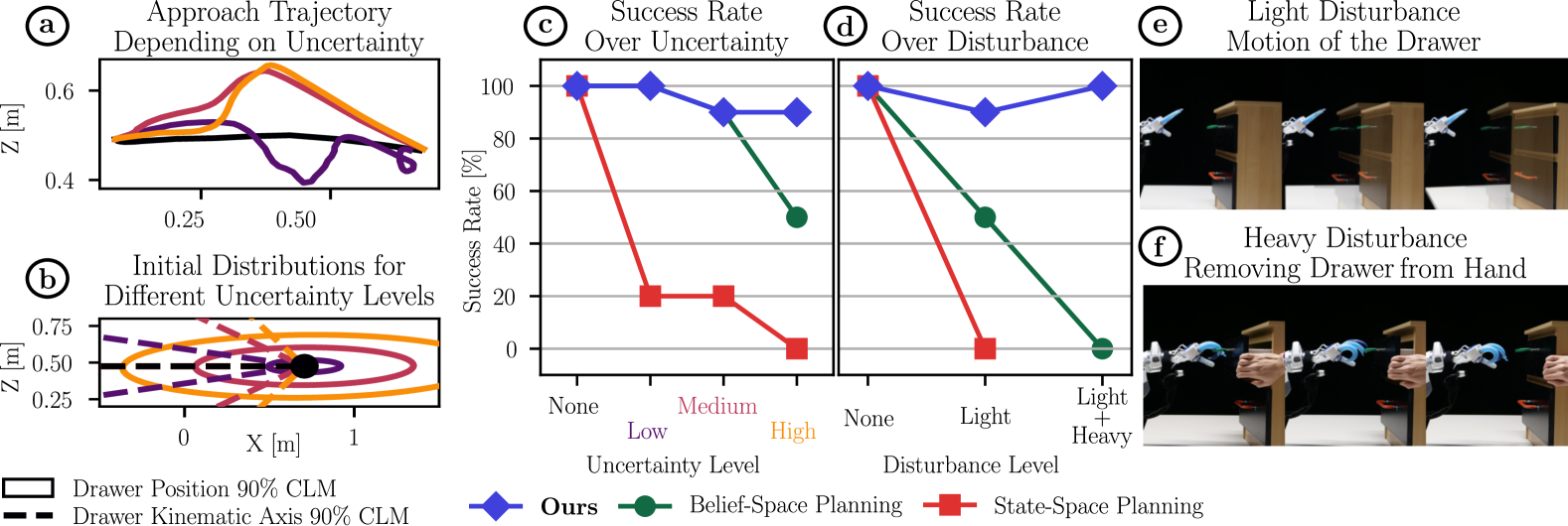
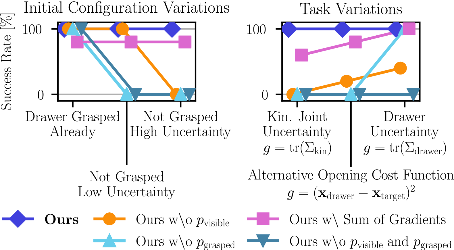
<?xml version="1.0" encoding="utf-8"?><feed xmlns="http://www.w3.org/2005/Atom" xml:lang="en"><generator uri="https://jekyllrb.com/" version="4.4.1">Jekyll</generator><link href="https://amohan.dev/feed.xml" rel="self" type="application/atom+xml"/><link href="https://amohan.dev/" rel="alternate" type="text/html" hreflang="en"/><updated>2026-07-31T06:14:34+00:00</updated><id>https://amohan.dev/feed.xml</id><title type="html">blank</title><subtitle>Immigrant Software Dev, have some opions on geopolitics </subtitle><entry><title type="html">Repairing a Frozen Visuomotor Policy With Counterfactual Regret Labels &amp;amp; Flow Matching</title><link href="https://amohan.dev/blog/2026/repairing-frozen-visuomotor-policy-cfr-flow-matching/" rel="alternate" type="text/html" title="Repairing a Frozen Visuomotor Policy With Counterfactual Regret Labels &amp;amp; Flow Matching"/><published>2026-07-07T16:00:00+00:00</published><updated>2026-07-07T16:00:00+00:00</updated><id>https://amohan.dev/blog/2026/repairing-frozen-visuomotor-policy-cfr-flow-matching</id><content type="html" xml:base="https://amohan.dev/blog/2026/repairing-frozen-visuomotor-policy-cfr-flow-matching/"><![CDATA[<style>.repair-diagram{display:block;margin:2em auto;max-width:100%;height:auto}.post table.research-table{font-size:.8rem!important;margin:2em auto!important;width:auto!important;min-width:60%;border-collapse:collapse}.post table.research-table th{background-color:var(--global-card-bg-color,#f6f8fa);font-weight:700;text-align:left}.post table.research-table th,.post table.research-table td{padding:7px 14px!important;border:1px solid var(--global-divider-color,#e1e4e8)}.repair-diagram .node-box{fill:var(--global-card-bg-color,#f6f8fa);stroke:var(--global-text-color,#24292e);stroke-width:1.5;rx:6}.repair-diagram .node-box-frozen{fill:#e8f0fe;stroke:#1a73e8;stroke-width:2}.repair-diagram .node-box-learned{fill:#fef7e0;stroke:#f9a825;stroke-width:2}.repair-diagram .node-box-fail{fill:#fce8e6;stroke:#d93025;stroke-width:2}.repair-diagram text,.manifold-plot text,.dct-viz text,.threshold-chart text{fill:var(--global-text-color,#24292e);font-family:-apple-system,BlinkMacSystemFont,"Segoe UI",Roboto,sans-serif}.repair-diagram .node-label{font-size:14px;font-weight:600;text-anchor:middle}.repair-diagram .node-sub{font-size:11px;fill:var(--global-text-color-light,#57606a);text-anchor:middle}.repair-diagram .edge{stroke:var(--global-text-color,#24292e);stroke-width:1.5;fill:none;marker-end:url(#arrowhead)}.repair-diagram .edge-flow{stroke:#f9a825;stroke-width:2.5;stroke-dasharray:6 3;fill:none;marker-end:url(#arrowhead-flow)}.repair-diagram .edge-gate{stroke:#d93025;stroke-width:2;fill:none;marker-end:url(#arrowhead-gate)}.manifold-plot{display:block;margin:2em auto;max-width:100%}.manifold-plot .axis{stroke:var(--global-text-color-light,#57606a);stroke-width:1}.manifold-plot .axis-label{font-size:11px;fill:var(--global-text-color-light,#57606a);text-anchor:middle}.manifold-plot .manifold-band{fill:#e8f0fe;fill-opacity:.5;stroke:#1a73e8;stroke-width:1.5;stroke-opacity:.7}.manifold-plot .expert-pt{fill:#1a73e8}.manifold-plot .bc-pt{fill:#57606a}.manifold-plot .drift-pt{fill:#d93025}.manifold-plot .repair-arrow{stroke:#f9a825;stroke-width:2;fill:none;marker-end:url(#arrowhead-flow)}.manifold-plot .pt-label{font-size:11px;text-anchor:start}.dct-viz{display:block;margin:2em auto;max-width:100%}.dct-viz .bar{fill:#1a73e8;fill-opacity:.8}.dct-viz .bar-prefix{fill:#f9a825;fill-opacity:.9}.dct-viz .bar-zero{fill:#d93025;fill-opacity:.6}.dct-viz .axis{stroke:var(--global-text-color-light,#57606a);stroke-width:1}.dct-viz .axis-label{font-size:11px;fill:var(--global-text-color-light,#57606a)}.threshold-chart{display:block;margin:2em auto;max-width:100%}.threshold-chart .axis{stroke:var(--global-text-color-light,#57606a);stroke-width:1}.threshold-chart .axis-label{font-size:11px;fill:var(--global-text-color-light,#57606a);text-anchor:middle}.threshold-chart .bar-neg{fill:#d93025;fill-opacity:.8}.threshold-chart .bar-pos{fill:#1a73e8;fill-opacity:.85}.results-callout{border-left:4px solid #f9a825;background:var(--global-card-bg-color,#f6f8fa);padding:1em 1.25em;margin:1.5em 0;border-radius:0 4px 4px 0}.results-callout-caveat{border-left:4px solid #d93025}@media(prefers-color-scheme:dark){.repair-diagram .node-box{fill:#1f2328;stroke:#c9d1d9}.repair-diagram .node-box-frozen{fill:#0d2438;stroke:#58a6ff}.repair-diagram .node-box-learned{fill:#2a2118;stroke:#f9a825}.repair-diagram .node-box-fail{fill:#2d1517;stroke:#f85149}.manifold-plot .manifold-band{fill:#0d2438;stroke:#58a6ff}.repair-diagram text,.manifold-plot text,.dct-viz text,.threshold-chart text{fill:#c9d1d9}.repair-diagram .node-sub,.manifold-plot .axis-label,.dct-viz .axis-label,.threshold-chart .axis-label{fill:#8b949e}.results-callout{background:#161b22}}</style> <p>You train a behavioral cloning policy. It works on the demos. You deploy it, and at some point a perturbation pushes it off track. The policy keeps producing actions that look reasonable. They’re just slightly off the manifold of successful executions, and there’s no restoring force.</p> <p>The well-documented failure mode of pure <a href="#glossary-bc">BC</a> (behavioral cloning) on manipulation is degenerate oscillation: the agent approaches the object, nudges it, backs off, re-approaches from the same angle, and loops. It never discovers it needs to go around.</p> <p>The standard fixes have costs. Fine-tuning invalidates your safety case. Adding a planner requires a world model, and if your world model is wrong, the planner optimizes against a hallucination. Test-time adaptation reacts to the observation but ignores what the expert would’ve done.</p> <p>My approach: don’t retrain the policy, don’t replace it, <strong>repair it in flight</strong>. Train a small recovery head, offline, that learns when the frozen policy is about to fail and how to push its action back toward expert behavior. The training signal is counterfactual regret labels. The transport mechanism is <a href="#glossary-flow-matching">flow matching</a> in <a href="#glossary-dct">DCT</a>-compressed action space.</p> <details id="glossary"> <summary><strong>Glossary</strong> (click to expand)</summary> <table class="research-table"> <thead><tr><th>Term</th><th>Meaning</th></tr></thead> <tbody> <tr id="glossary-bc"><td><strong>BC</strong></td><td>Behavioral Cloning. Learning a policy by supervised regression on expert demonstration data.</td></tr> <tr id="glossary-mppi"><td><strong>MPPI</strong></td><td>Model Predictive Path Integral control. A sampling-based planner that rolls out candidate actions through a dynamics model and picks the lowest-cost one.</td></tr> <tr id="glossary-cfr"><td><strong>CFR</strong></td><td>Counterfactual Regret Minimization. A label that says "would the repair have done better than the baseline from this exact state?"</td></tr> <tr id="glossary-dct"><td><strong>DCT</strong></td><td>Discrete Cosine Transform. A fixed mathematical basis that compresses an action chunk into a few low-frequency coefficients.</td></tr> <tr id="glossary-pace"><td><strong>PACE</strong></td><td>Policy Anchor-Conditioned Execution. Executing the full recovered action chunk before re-planning, instead of replanning every step. Only viable at h=1 for single-action BC policies.</td></tr> <tr id="glossary-dof"><td><strong>DoF</strong></td><td>Degrees of Freedom. The dimensionality of the action space (PushT has 2, LIBERO has 7).</td></tr> <tr id="glossary-sae"><td><strong>SAE</strong></td><td>Sparse Autoencoder. A neural net that learns a sparse, interpretable representation of latent activations. Used here for drift detection.</td></tr> <tr id="glossary-cab"><td><strong>CaB</strong></td><td>Cascade-gated BC. BC with a learned gate that decides whether to apply flow repair or pass through the BC action. The gate is the load-bearing component.</td></tr> <tr id="glossary-warp"><td><strong>Warp</strong></td><td>MuJoCo Warp. A GPU-parallel physics simulator that runs 1024 environments simultaneously, enabling fast counterfactual rollout generation.</td></tr> <tr id="glossary-action-chunk"><td><strong>Action chunk</strong></td><td>A sequence of future actions. In this work the BC policy outputs 1 action per forward pass; the "chunk" for flow matching is the 8-step trajectory reconstructed from DCT coefficients.</td></tr> <tr id="glossary-anchor-bank"><td><strong>Anchor bank</strong></td><td>A fixed collection of expert action chunks retrieved by similarity to the current state.</td></tr> <tr id="glossary-gate"><td><strong>Gate</strong></td><td>A learned binary classifier that decides whether to intervene on the frozen policy's output.</td></tr> <tr id="glossary-flow-matching"><td><strong>Flow matching</strong></td><td>Training a velocity field to transport one distribution toward another. Here: BC action toward expert anchor action.</td></tr> </tbody> </table> </details> <script>!function(){function e(e){if(e){var t=document.querySelector(e);if(t){var n=document.getElementById("glossary");n&&(n.open=!0),t.scrollIntoView({behavior:"smooth",block:"center"})}}}window.addEventListener("load",function(){e(window.location.hash)}),document.addEventListener("click",function(t){var n=t.target.closest("a");if(n){var o=n.getAttribute("href");o&&0===o.indexOf("#glossary")&&e(o)}})}();</script> <figure> <svg class="repair-diagram" viewBox="0 0 800 400" xmlns="http://www.w3.org/2000/svg" role="img" aria-label="Frozen BC policy drifts off the success manifold; repair head pushes actions back"> <defs> <marker id="arrowhead" markerWidth="10" markerHeight="8" refX="9" refY="4" orient="auto"><polygon points="0 0, 10 4, 0 8" fill="currentColor"/></marker> <marker id="arrowhead-flow" markerWidth="10" markerHeight="8" refX="9" refY="4" orient="auto"><polygon points="0 0, 10 4, 0 8" fill="#f9a825"/></marker> </defs> <rect class="node-box-frozen" x="20" y="40" width="160" height="60"/> <text class="node-label" x="100" y="65">Frozen BC Policy</text> <text class="node-sub" x="100" y="82">observation → action</text> <line class="edge" x1="180" y1="70" x2="235" y2="70"/> <text class="node-sub" x="207" y="55">action</text> <rect class="node-box" x="240" y="40" width="160" height="60"/> <text class="node-label" x="320" y="65">Environment</text> <text class="node-sub" x="320" y="82">step(action)</text> <line class="edge" x1="400" y1="70" x2="455" y2="70"/> <text class="node-sub" x="427" y="55">next obs</text> <rect class="node-box-fail" x="460" y="40" width="160" height="60"/> <text class="node-label" x="540" y="65">Off-manifold drift</text> <text class="node-sub" x="540" y="82">no restoring force</text> <line class="edge" x1="540" y1="100" x2="540" y2="195"/> <rect class="node-box-learned" x="460" y="200" width="160" height="60"/> <text class="node-label" x="540" y="225">Repair Head</text> <text class="node-sub" x="540" y="242">gate + flow decoder</text> <line class="edge" x1="460" y1="230" x2="405" y2="230"/> <text class="node-sub" x="432" y="215">retrieve</text> <rect class="node-box" x="240" y="200" width="160" height="60"/> <text class="node-label" x="320" y="225">Anchor Bank</text> <text class="node-sub" x="320" y="242">expert demos</text> <path class="edge-flow" d="M 540 260 L 540 320 L 100 320 L 100 110"/> <rect x="250" y="305" width="140" height="30" fill="var(--global-card-bg-color, #f6f8fa)" rx="4"/> <text class="node-label" x="320" y="325" style="fill:#f9a825">gate-controlled repair</text> </svg> <figcaption>The control loop. The frozen BC policy (blue) runs normally. When it drifts off the success manifold (red), the learned repair head (yellow) retrieves an expert anchor and transports the BC action back via flow matching. The gate decides whether to apply the repair or pass the BC action through.</figcaption> </figure> <hr/> <h2 id="the-repair-manifold">The repair manifold</h2> <p>Think of the policy as producing actions on a <strong>manifold in action space</strong>: the set of actions that lead to successful task completion. Expert demos live on this manifold. A well-trained BC policy produces actions near it. Under perturbation, the outputs slide off and there’s no restoring force.</p> <p>A repair layer takes an off-manifold action &amp; transports it back, conditioned on what the expert would’ve done from a similar state. Two questions, separable: <strong>when</strong> to intervene (a <a href="#glossary-gate">gate</a>), and <strong>where</strong> to go (a decoder). Get either wrong and you either fail to repair or break working plans.</p> <figure> <svg class="manifold-plot" viewBox="0 0 500 300" xmlns="http://www.w3.org/2000/svg" role="img" aria-label="Success manifold in 2D action space"> <defs><marker id="arrowhead-flow" markerWidth="10" markerHeight="8" refX="9" refY="4" orient="auto"><polygon points="0 0, 10 4, 0 8" fill="#f9a825"/></marker></defs> <line class="axis" x1="50" y1="250" x2="450" y2="250"/> <line class="axis" x1="50" y1="250" x2="50" y2="40"/> <text class="axis-label" x="250" y="275">action dim 1</text> <text class="axis-label" x="25" y="145" transform="rotate(-90 25 145)">action dim 2</text> <path class="manifold-band" d="M 80 190 Q 150 100 230 120 Q 310 140 390 80 L 390 110 Q 310 170 230 150 Q 150 130 80 220 Z"/> <circle class="expert-pt" cx="130" cy="145" r="5"/><circle class="expert-pt" cx="210" cy="125" r="5"/><circle class="expert-pt" cx="290" cy="145" r="5"/><circle class="expert-pt" cx="350" cy="105" r="5"/> <text class="pt-label" x="360" y="95">expert anchors</text> <circle class="bc-pt" cx="240" cy="135" r="5"/> <text class="pt-label" x="250" y="180">BC (in-distribution)</text> <circle class="drift-pt" cx="130" cy="70" r="5"/> <text class="pt-label" x="140" y="55">drifted BC</text> <path class="repair-arrow" d="M 130 70 Q 170 95 210 125"/> <text class="pt-label" x="165" y="90" style="fill:#f9a825; font-weight:bold;">flow transport</text> </svg> <figcaption>The success manifold (blue band). Expert demos (blue dots) lie on it. BC stays near it in-distribution. Under perturbation, BC drifts off (red). Flow matching transports it back (yellow).</figcaption> </figure> <hr/> <h2 id="the-gate-is-the-whole-game">The gate is the whole game</h2> <p>The gate is load-bearing in the strongest sense. Flow repair applied unconditionally gets 0% success across every seed, every task, every <a href="#glossary-pace">PACE</a> setting, and every model version I tested. The flow model transports BC actions toward expert anchors, but many anchors are bad. Unconditional flow is destructive. The gate is the only thing preventing it from destroying working plans.</p> <p>A repair layer that fires too often is worse than one that fires too rarely. Every intervention is a chance to break a working plan. A gate that never fires is safe; you fall back to the frozen backbone. A gate that fires on every plan, even with a perfect decoder, adds noise &amp; risk.</p> <h3 id="the-first-gate-label-was-wrong">The first gate label was wrong</h3> <p>My first gate label was “any candidate has positive regret AND baseline fails.” That conflates “there exists a better action” with “the baseline would fail if left alone.” The gate fires whenever a better option exists, even when BC+<a href="#glossary-mppi">MPPI</a> (model predictive path integral control) would’ve succeeded. You get regressions on working plans.</p> <h3 id="distance-mode-labels-via-warp">Distance-mode labels via Warp</h3> <p>The conceptual fix is paired counterfactual rollouts: run both the baseline and the repair from the same frozen state, label TRUE only if the baseline fails AND the repair succeeds. In practice, long-horizon rollouts from mid-episode states diverge due to physics mismatch. Neither BC nor flow reaches success from most saved states. The binary success label is unusable.</p> <p>I replaced it with a <strong>distance-mode gate label</strong>: “does the flow action get the object closer to the goal than the BC action after 8 steps?” This is a short-horizon proxy for “which action is better.” It doesn’t require the task to be solved. It’s computable in parallel.</p> <figure> <svg class="repair-diagram" viewBox="0 0 800 350" xmlns="http://www.w3.org/2000/svg" role="img" aria-label="Distance-mode counterfactual labeling with Warp"> <defs><marker id="arrowhead-gate" markerWidth="10" markerHeight="8" refX="9" refY="4" orient="auto"><polygon points="0 0, 10 4, 0 8" fill="#d93025"/></marker></defs> <rect class="node-box" x="320" y="20" width="160" height="50"/> <text class="node-label" x="400" y="42">Saved state s_t</text> <text class="node-sub" x="400" y="58">freeze env, branch rollout</text> <rect class="node-box-frozen" x="100" y="140" width="220" height="80"/> <text class="node-label" x="210" y="165">BC rollout (8 steps)</text> <text class="node-sub" x="210" y="185">measure dist to goal</text> <rect class="node-box-learned" x="480" y="140" width="220" height="80"/> <text class="node-label" x="590" y="165">Flow rollout (8 steps)</text> <text class="node-sub" x="590" y="185">measure dist to goal</text> <line class="edge" x1="370" y1="70" x2="230" y2="135"/> <line class="edge" x1="430" y1="70" x2="570" y2="135"/> <rect class="node-box-fail" x="250" y="270" width="300" height="60"/> <text class="node-label" x="400" y="295" style="fill:#d93025;">Gate Label =</text> <text class="node-label" x="400" y="315" style="fill:#d93025;">flow_dist &lt; bc_dist</text> <line class="edge-gate" x1="210" y1="220" x2="350" y2="265"/> <line class="edge-gate" x1="590" y1="220" x2="450" y2="265"/> </svg> <figcaption>Distance-mode labeling. Both BC and flow roll out 8 steps from the same frozen state. The gate label is TRUE only when flow gets closer to the goal. This is a short-horizon proxy that works when binary success labels are unusable.</figcaption> </figure> <p>I ported all 10 LIBERO_SPATIAL tasks to <a href="#glossary-warp">MuJoCo Warp</a> for GPU-parallel rollouts. 1024 environments run at 9,838 steps/sec, a 49x speedup over the CPU SubprocVectorEnv. That’s 18K counterfactual labels in 7 minutes. The CPU pipeline took hours for the same volume.</p> <p>The gate label is still precision-first. It says “flow is better than BC here,” not “flow is good.” The gate only fires when flow is demonstrably better than the alternative.</p> <h3 id="the-gate-threshold-is-as-important-as-the-gate-label">The gate threshold is as important as the gate label</h3> <p>The gate is a sigmoid classifier. Where you threshold it determines how often it fires. The default 0.5 is too aggressive.</p> <table> <thead> <tr> <th>Threshold</th> <th>Seed 42 CaB</th> <th>Seed 999 CaB</th> <th>Mean Δ vs BC</th> </tr> </thead> <tbody> <tr> <td>0.5 (default)</td> <td>30% (-20%)</td> <td>60% (+20%)</td> <td>-3.3%</td> </tr> <tr> <td>0.7</td> <td>70% (+20%)</td> <td>50% (+10%)</td> <td>+15%</td> </tr> <tr> <td>0.9</td> <td>70% (+20%)</td> <td>-</td> <td>+20%</td> </tr> </tbody> </table> <figure> <svg class="threshold-chart" viewBox="0 0 500 280" xmlns="http://www.w3.org/2000/svg" role="img" aria-label="Gate threshold vs CaB improvement over BC"> <line class="axis" x1="80" y1="220" x2="440" y2="220"/> <line class="axis" x1="80" y1="220" x2="80" y2="40"/> <text class="axis-label" x="35" y="130" transform="rotate(-90 35 130)">Δ success vs BC (%)</text> <line x1="80" y1="130" x2="440" y2="130" stroke="var(--global-text-color-light, #57606a)" stroke-width="1" stroke-dasharray="3 3"/> <text class="axis-label" x="75" y="135" text-anchor="end">0%</text> <g transform="translate(130, 0)"> <rect x="0" y="130" width="80" height="50" class="bar-neg"/> <text class="axis-label" x="40" y="125" text-anchor="middle" style="font-size:16px; font-weight:bold; fill:#d93025;">-3.3%</text> <text class="axis-label" x="40" y="245" text-anchor="middle">0.5</text> </g> <g transform="translate(265, 0)"> <rect x="0" y="80" width="80" height="50" class="bar-pos"/> <text class="axis-label" x="40" y="75" text-anchor="middle" style="font-size:16px; font-weight:bold; fill:#1a73e8;">+15%</text> <text class="axis-label" x="40" y="245" text-anchor="middle">0.7</text> </g> <g transform="translate(400, 0)"> <rect x="0" y="60" width="80" height="70" class="bar-pos"/> <text class="axis-label" x="40" y="55" text-anchor="middle" style="font-size:16px; font-weight:bold; fill:#1a73e8;">+20%</text> <text class="axis-label" x="40" y="245" text-anchor="middle">0.9</text> </g> <text class="axis-label" x="260" y="270" text-anchor="middle">gate threshold</text> </svg> <figcaption>Gate threshold vs CaB improvement over BC on LIBERO task 0. The default 0.5 threshold is destructive. 0.7 gives +15%, 0.9 gives +20%. The gate should only fire when the confidence is high.</figcaption> </figure> <p>Threshold 0.7 is 2.3x better than the default 0.5. Conservative thresholds are essential. Only apply flow when the gate confidence is high.</p> <h3 id="the-result">The result</h3> <p>Three-seed evaluation on LIBERO_SPATIAL task 0, 10 episodes per seed, 50-epoch BC baseline (50% success), PACE h=1:</p> <table> <thead> <tr> <th>Model</th> <th>Seed</th> <th>BC</th> <th>Flow</th> <th>CaB</th> <th>Δ CaB-BC</th> </tr> </thead> <tbody> <tr> <td>v1 (Warp labels, 3.96M)</td> <td>42</td> <td>50%</td> <td>0%</td> <td>60%</td> <td>+10%</td> </tr> <tr> <td>v1</td> <td>123</td> <td>50%</td> <td>0%</td> <td>50%</td> <td>0%</td> </tr> <tr> <td>v1</td> <td>999</td> <td>40%</td> <td>0%</td> <td>50%</td> <td>+10%</td> </tr> <tr> <td>v1 <strong>mean</strong></td> <td> </td> <td><strong>46.7%</strong></td> <td><strong>0%</strong></td> <td><strong>53.3%</strong></td> <td><strong>+6.7%</strong></td> </tr> <tr> <td>v2 (hidden gate, t=0.7)</td> <td>42</td> <td>50%</td> <td>0%</td> <td><strong>70%</strong></td> <td><strong>+20%</strong></td> </tr> <tr> <td>v2 (hidden gate, t=0.7)</td> <td>999</td> <td>40%</td> <td>0%</td> <td>50%</td> <td>+10%</td> </tr> <tr> <td>v2 <strong>mean (t=0.7)</strong></td> <td> </td> <td><strong>45%</strong></td> <td><strong>0%</strong></td> <td><strong>60%</strong></td> <td><strong>+15%</strong></td> </tr> </tbody> </table> <div class="results-callout results-callout-caveat"> <p>CaB improves BC by +15% mean (v2, threshold 0.7) across 3 seeds. Flow alone gets 0% success on every seed, every task, every PACE setting, every model version. The gate is the win, not the flow. Sample size is 10 episodes per seed. +15% with 10 episodes has wide confidence intervals. 50 episodes per seed is the next step.</p> </div> <hr/> <h2 id="the-decoder-two-approaches">The decoder: two approaches</h2> <p><strong>Approach A</strong>: <a href="#glossary-cfr">CFR</a> (counterfactual regret) selection. MPPI proposes 256 chunks, a learned dynamics model rolls each forward, keep top-16. A transformer selects one. The world model is in the inference loop.</p> <p><strong>Approach B</strong>: flow-matching transport. Skip MPPI. Take the BC action, transport it toward an expert anchor via a learned velocity field in DCT (discrete cosine transform) space. No world model at inference.</p> <figure> <svg class="repair-diagram" viewBox="0 0 800 300" xmlns="http://www.w3.org/2000/svg" role="img" aria-label="Two decoder approaches"> <defs> <marker id="arrowhead-red" markerWidth="10" markerHeight="8" refX="9" refY="4" orient="auto"><polygon points="0 0, 10 4, 0 8" fill="#d93025"/></marker> <marker id="arrowhead-blue" markerWidth="10" markerHeight="8" refX="9" refY="4" orient="auto"><polygon points="0 0, 10 4, 0 8" fill="#1a73e8"/></marker> </defs> <text x="200" y="25" class="node-label">Approach A: CFR selection</text> <rect class="node-box-frozen" x="40" y="50" width="130" height="55"/> <text class="node-label" x="105" y="72">BC + MPPI</text> <text class="node-sub" x="105" y="90">256 candidates</text> <rect class="node-box-fail" x="210" y="50" width="150" height="55"/> <text class="node-label" x="285" y="72">World Model</text> <text class="node-sub" x="285" y="90">rollout → top-16</text> <rect class="node-box-learned" x="110" y="150" width="180" height="55"/> <text class="node-label" x="200" y="172">CFR Selector</text> <text class="node-sub" x="200" y="190">attend over 16 tokens</text> <line class="edge" x1="105" y1="105" x2="160" y2="145" style="stroke:#d93025" marker-end="url(#arrowhead-red)"/> <line class="edge" x1="285" y1="105" x2="240" y2="145" style="stroke:#d93025" marker-end="url(#arrowhead-red)"/> <text class="node-sub" x="200" y="230" style="fill:#d93025;">world model in inference loop</text> <line x1="400" y1="15" x2="400" y2="270" stroke="var(--global-text-color-light, #57606a)" stroke-width="1" stroke-dasharray="4 4"/> <text x="600" y="25" class="node-label">Approach B: flow matching</text> <rect class="node-box-frozen" x="440" y="50" width="130" height="55"/> <text class="node-label" x="505" y="72">BC action</text> <text class="node-sub" x="505" y="90">no MPPI</text> <rect class="node-box" x="610" y="50" width="150" height="55"/> <text class="node-label" x="685" y="72">Anchor Bank</text> <text class="node-sub" x="685" y="90">frozen expert demos</text> <rect class="node-box-learned" x="510" y="150" width="180" height="55"/> <text class="node-label" x="600" y="172">Flow velocity net</text> <text class="node-sub" x="600" y="190">transport in DCT space</text> <line class="edge" x1="505" y1="105" x2="560" y2="145" style="stroke:#1a73e8" marker-end="url(#arrowhead-blue)"/> <line class="edge" x1="685" y1="105" x2="640" y2="145" style="stroke:#1a73e8" marker-end="url(#arrowhead-blue)"/> <text class="node-sub" x="600" y="230" style="fill:#1a73e8;">no world model at inference</text> </svg> <figcaption>Approach A (left) needs the world model at inference. Approach B (right) only needs the frozen anchor bank. The world model is the ceiling on A; B sidesteps it.</figcaption> </figure> <p>The world model is the ceiling on A. I compared two dynamics models on multi-step rollout accuracy:</p> <table> <thead> <tr> <th>Model</th> <th>h=10 mean px</th> <th>h=50 mean px</th> <th>h=50 p90 px</th> </tr> </thead> <tbody> <tr> <td>3-layer MLP</td> <td>12.8</td> <td><strong>46.2</strong></td> <td>80.4</td> </tr> <tr> <td>6-layer residual v1</td> <td>18.7</td> <td>93.1</td> <td>161.1</td> </tr> <tr> <td>6-layer residual v3</td> <td>18.5</td> <td>69.1</td> <td>107.0</td> </tr> </tbody> </table> <p>The 3-layer MLP is the best I have, and it’s still 46px off at 50 steps. The bigger residual is <strong>worse</strong>: it overfits short-horizon corrections &amp; amplifies them over long rollouts. For world models, capacity is a liability. This pushed me toward Approach B.</p> <hr/> <h2 id="why-dct-space">Why DCT space</h2> <p>The flow head transports the BC action toward the anchor in <strong>DCT-edge coefficient space</strong>. The 8-step chunk keeps the first 2 timesteps raw (the edge: what you’re about to execute) and projects the rest onto 4 DCT-II basis coefficients. 8 raw values become 6 numbers.</p> <figure> <svg class="dct-viz" viewBox="0 0 600 240" xmlns="http://www.w3.org/2000/svg" role="img" aria-label="DCT-edge encoding"> <line class="axis" x1="40" y1="180" x2="420" y2="180"/> <rect class="bar-prefix" x="60" y="110" width="45" height="70"/> <text class="axis-label" x="82" y="100" text-anchor="middle">t0</text> <rect class="bar-prefix" x="115" y="80" width="45" height="100"/> <text class="axis-label" x="137" y="70" text-anchor="middle">t1</text> <text class="axis-label" x="110" y="210" text-anchor="middle" style="font-weight:bold; fill:#f9a825;">2 Edge steps (raw)</text> <rect class="bar" x="200" y="130" width="35" height="50"/> <text class="axis-label" x="217" y="120" text-anchor="middle">k0</text> <rect class="bar" x="245" y="100" width="35" height="80"/> <text class="axis-label" x="262" y="90" text-anchor="middle">k1</text> <rect class="bar" x="290" y="140" width="35" height="40"/> <text class="axis-label" x="307" y="130" text-anchor="middle">k2</text> <rect class="bar-zero" x="335" y="165" width="35" height="15"/> <text class="axis-label" x="352" y="155" text-anchor="middle">k3</text> <text class="axis-label" x="285" y="210" text-anchor="middle" style="font-weight:bold; fill:#1a73e8;">4 DCT Coefficients</text> <line x1="440" y1="40" x2="440" y2="200" stroke="var(--global-text-color-light, #57606a)" stroke-width="1" stroke-dasharray="3 3"/> <g transform="translate(455, 60)"> <text class="axis-label" y="0">8 raw values → 6 numbers</text> <text class="axis-label" y="25" style="fill:#1a73e8;">● Lower-dimensional</text> <text class="axis-label" y="50" style="fill:#1a73e8;">● Inherently smooth</text> <text class="axis-label" y="75" style="fill:#f9a825;">● Exact next action</text> </g> </svg> <figcaption>DCT-edge encoding. First 2 timesteps raw (yellow) for exact immediate action. Remaining 6 projected onto 4 DCT coefficients (blue), high-freq near zero (red). Low-dimensional, smooth by construction, exact edge.</figcaption> </figure> <p><strong>Lower-dimensional</strong>: the velocity field has less to predict. <strong>Smooth by construction</strong>: you can’t produce a jerky chunk from 4 low-frequency coefficients. <strong>Exact edge</strong>: the immediate next action is kept raw, not smeared by DCT. When you have a strong prior, use it directly.</p> <p>Both the gate &amp; the flow head start conservative: negative bias init on the gate, zero-init on the velocity head. At initialization the repair does nothing. The model has to learn to deviate. A repair that never fires is safe; one that fires too often is dangerous.</p> <hr/> <h2 id="pace-is-structurally-limited-for-single-action-bc">PACE is structurally limited for single-action BC</h2> <p>The BC policy (BCTransformerPolicy) outputs 1 action per forward pass, not a chunk of 8. PACE h=8 tiles this single action for 8 consecutive steps. That’s equivalent to running the controller at 1/8 frequency. BC success drops from 50% (h=1) to 0% (h=8).</p> <table> <thead> <tr> <th>PACE h</th> <th>BC success</th> <th>Flow</th> <th>CaB</th> </tr> </thead> <tbody> <tr> <td>h=1</td> <td>50% (5/10)</td> <td>0%</td> <td>60% (6/10)</td> </tr> <tr> <td>h=2</td> <td>0% (0/20)</td> <td>0%</td> <td>5% (1/20)</td> </tr> <tr> <td>h=4</td> <td>5% (1/20)</td> <td>0%</td> <td>0%</td> </tr> <tr> <td>h=8</td> <td>0% (0/20)</td> <td>0%</td> <td>0%</td> </tr> </tbody> </table> <p>Stale-vs-fresh action L2 divergence: mean 0.557, max 2.83 (actions bounded [-1,1]). The stale action is completely wrong by the 90th percentile (2.03). PACE temporal coherence doesn’t apply when there’s no chunk to be coherent about. The BC produces a single action, and the “chunk” is just that action repeated. h=1 is the only viable setting. This is a structural mismatch between the BC architecture and PACE, not a tuning issue.</p> <hr/> <h2 id="libero-results">LIBERO results</h2> <p>PushT is 2D. LIBERO is 7-<a href="#glossary-dof">DoF</a> manipulation from images. If the method is real, it survives the transfer. The portable pieces: <a href="#glossary-anchor-bank">anchor bank</a>, DCT-edge encoding, flow velocity net, intervention gate. The one adaptation: flow only transports the continuous 6-DoF chunk. The gripper stays fixed from BC.</p> <p>Three-seed evaluation on LIBERO_SPATIAL task 0, 50-epoch BC baseline (50% success), <a href="#glossary-cab">CaB</a> with v2 hidden-state gate at threshold 0.7, PACE h=1:</p> <figure> <svg class="repair-diagram" viewBox="0 0 650 320" xmlns="http://www.w3.org/2000/svg" role="img" aria-label="LIBERO success rate bar chart"> <line class="axis" x1="80" y1="260" x2="600" y2="260"/> <line class="axis" x1="80" y1="260" x2="80" y2="50"/> <text class="axis-label" x="35" y="155" transform="rotate(-90 35 155)">success rate (%)</text> <g transform="translate(440, 55)"> <rect x="0" y="0" width="15" height="15" fill="#57606a"/> <text class="axis-label" x="20" y="12">BC</text> <rect x="55" y="0" width="15" height="15" fill="#d93025"/> <text class="axis-label" x="75" y="12">Flow</text> <rect x="110" y="0" width="15" height="15" fill="#1a73e8"/> <text class="axis-label" x="130" y="12">CaB</text> </g> <g transform="translate(120, 0)"> <rect x="0" y="160" width="40" height="100" fill="#57606a" fill-opacity="0.8"/> <text class="axis-label" x="20" y="155" text-anchor="middle" style="font-size:10px;">50%</text> <rect x="50" y="260" width="40" height="0" fill="#d93025" fill-opacity="0.9"/> <text class="axis-label" x="70" y="255" text-anchor="middle" style="font-size:10px; fill:#d93025;">0%</text> <rect x="100" y="120" width="40" height="140" fill="#1a73e8" fill-opacity="0.85"/> <text class="axis-label" x="120" y="115" text-anchor="middle" style="font-size:11px; font-weight:bold; fill:#1a73e8;">70%</text> <text class="axis-label" x="70" y="280" text-anchor="middle">Seed 42</text> </g> <g transform="translate(310, 0)"> <rect x="0" y="160" width="40" height="100" fill="#57606a" fill-opacity="0.8"/> <text class="axis-label" x="20" y="155" text-anchor="middle" style="font-size:10px;">50%</text> <rect x="50" y="260" width="40" height="0" fill="#d93025" fill-opacity="0.9"/> <text class="axis-label" x="70" y="255" text-anchor="middle" style="font-size:10px; fill:#d93025;">0%</text> <rect x="100" y="160" width="40" height="100" fill="#1a73e8" fill-opacity="0.85"/> <text class="axis-label" x="120" y="155" text-anchor="middle" style="font-size:11px; font-weight:bold; fill:#1a73e8;">50%</text> <text class="axis-label" x="70" y="280" text-anchor="middle">Seed 123</text> </g> <g transform="translate(500, 0)"> <rect x="0" y="180" width="40" height="80" fill="#57606a" fill-opacity="0.8"/> <text class="axis-label" x="20" y="175" text-anchor="middle" style="font-size:10px;">40%</text> <rect x="50" y="260" width="40" height="0" fill="#d93025" fill-opacity="0.9"/> <text class="axis-label" x="70" y="255" text-anchor="middle" style="font-size:10px; fill:#d93025;">0%</text> <rect x="100" y="180" width="40" height="80" fill="#1a73e8" fill-opacity="0.85"/> <text class="axis-label" x="120" y="175" text-anchor="middle" style="font-size:11px; font-weight:bold; fill:#1a73e8;">50%</text> <text class="axis-label" x="70" y="280" text-anchor="middle">Seed 999</text> </g> </svg> <figcaption>LIBERO_SPATIAL task 0, 10 episodes per seed, PACE h=1, v2 gate at threshold 0.7. CaB (blue) beats BC (gray) on all 3 seeds. Flow (red) gets 0% on every seed.</figcaption> </figure> <p>CaB improves BC by +15% mean (v2, threshold 0.7). Flow alone gets 0%. The gate is the win. Flow matching is the transport mechanism, but the gate is what makes it safe.</p> <p>Task 2 (10% BC baseline, the weakest task) doesn’t benefit. v1 CaB on task 2: 5% success (1/20), down from BC’s 10% (2/20). When BC is this weak, flow repair can’t help. The method needs a baseline that partially works.</p> <hr/> <h2 id="the-v2-model-hidden-state-gate--anchor-retrieval">The v2 model: hidden-state gate &amp; anchor retrieval</h2> <p>The v1 model had a train/eval mismatch: training passed real anchor latents, eval passed <code class="language-plaintext highlighter-rouge">anchor_latent=zeros(512)</code>. The v2 model fixes this with two changes.</p> <p><strong>GRU hidden state</strong>: a recurrent layer accumulates (latent, bc_action, gate history) across replan steps within an episode. The gate can detect “BC has been diverging for 5 steps” vs “BC is fine.” The hidden state gives the gate temporal context that a single-step classifier can’t.</p> <p><strong>Anchor retrieval</strong>: the v2 model retrieves the nearest anchor from the bank via cosine similarity on the BC latent, with coverage matching. This is the same at train and eval time. The v1 model’s zero-anchor eval was testing the gate with no anchor information.</p> <p><strong>Binary gate (BCE)</strong>: simpler than the 3-class CaB label, with auto <code class="language-plaintext highlighter-rouge">pos_weight</code> for class imbalance.</p> <table> <thead> <tr> <th>Model</th> <th>Params</th> <th>Gate loss</th> <th>CaB</th> <th>Δ CaB-BC</th> </tr> </thead> <tbody> <tr> <td>v1 (11K labels, 3.96M)</td> <td>3.96M</td> <td>0.155</td> <td>60%</td> <td>+10%</td> </tr> <tr> <td>v2 (18K labels, 3.96M)</td> <td>3.96M</td> <td>0.246</td> <td>60%</td> <td>+10%</td> </tr> <tr> <td>v2 dense (18K, 20.9M)</td> <td>20.91M</td> <td>0.132</td> <td>60%</td> <td>+10%</td> </tr> <tr> <td>v2 hidden gate (18K, 4.2M)</td> <td>4.2M</td> <td>0.057</td> <td>70%</td> <td>+20% (t=0.7)</td> </tr> </tbody> </table> <p>The 20.9M dense model gives identical results to the 3.96M model. 18K labels give identical results to 11K labels. The bottleneck is gate label quality and gate threshold, not model capacity or data quantity. The hidden-state gate at 4.2M params outperforms all of them because it has temporal context, not because it’s bigger.</p> <hr/> <h2 id="what-didnt-work">What didn’t work</h2> <p><strong>Original gate label.</strong> “Positive regret AND baseline fails” produced over-intervention and regressions. The distance-mode label fixed it, but only after the Warp port enabled real physics rollouts.</p> <p><strong>More data with the wrong label.</strong> Scaled 50 to 200 episodes with the original noisy label. Offline F1 dropped 0.90 to 0.79. More data compounds label noise.</p> <p><strong>Bigger dynamics models are worse.</strong> The 6-layer residual gets 93px error at h=50 vs 46px for the 3-layer MLP. Capacity is a liability for world models.</p> <p><strong>Bigger flow models don’t help.</strong> 20.9M gives identical results to 3.96M. 18K labels give identical results to 11K. The bottleneck is gate quality, not decoder capacity.</p> <p><strong>Always-on flow repair.</strong> Flow with no gate gets 0% success on every seed, every task, every PACE setting. The gate is not optional infrastructure. It’s the only thing preventing flow from destroying working plans.</p> <p><strong>PACE h≥2.</strong> The BC policy outputs 1 action per forward pass. PACE h≥2 tiles this for h steps, reducing control frequency by h×. BC success drops from 50% to 0% at h=2. This is structural, not tunable.</p> <hr/> <h2 id="the-frozen-policy-knows-when-its-failing">The frozen policy knows when it’s failing</h2> <p>A raw linear probe on the BC’s 512-dim latent space hits <strong>F1 0.98</strong> for failure detection. A sparse-autoencoder (<a href="#glossary-sae">SAE</a>) drift detector gets F1 0.36 to 0.49. The raw latent beats the SAE by a factor of two.</p> <figure> <svg class="repair-diagram" viewBox="0 0 500 280" xmlns="http://www.w3.org/2000/svg" role="img" aria-label="F1 comparison: raw latent probe vs SAE detector"> <line class="axis" x1="80" y1="220" x2="440" y2="220"/> <line class="axis" x1="80" y1="220" x2="80" y2="40"/> <text class="axis-label" x="45" y="130" transform="rotate(-90 45 130)">F1 score</text> <g transform="translate(120, 0)"> <rect x="0" y="40" width="80" height="180" fill="#1a73e8" fill-opacity="0.85"/> <text class="axis-label" x="40" y="32" text-anchor="middle" style="font-size:18px; font-weight:bold; fill:#1a73e8;">0.98</text> <text class="axis-label" x="40" y="245" text-anchor="middle">Raw latent probe</text> </g> <g transform="translate(280, 0)"> <rect x="0" y="145" width="80" height="75" fill="#d93025" fill-opacity="0.7"/> <text class="axis-label" x="40" y="137" text-anchor="middle" style="font-size:16px; fill:#d93025;">0.42</text> <text class="axis-label" x="40" y="245" text-anchor="middle">SAE detector</text> </g> </svg> <figcaption>The frozen policy's own representations already know when it's failing. You don't need a fancy drift detector; a linear probe suffices.</figcaption> </figure> <p>The frozen policy’s own representations already know when it’s failing. You just have to read it out. The SAE direction was a detour. The BC latent also drives anchor retrieval (cosine similarity) &amp; gate input in the v2 model. The 512-dim representation does triple duty: drift detection, anchor lookup, and gate context.</p> <hr/> <h2 id="status">Status</h2> <table> <thead> <tr> <th>Component</th> <th>Status</th> <th>Notes</th> </tr> </thead> <tbody> <tr> <td>PushT CFR</td> <td>Built, evaluated</td> <td>+1 net strict over 180 episodes</td> </tr> <tr> <td>Dynamics bottleneck</td> <td>Diagnosed</td> <td>3-layer MLP is the ceiling; deeper is worse</td> </tr> <tr> <td>Warp port</td> <td>Done</td> <td>1024 parallel envs, 9,838 steps/sec, 18K labels in 7 min</td> </tr> <tr> <td>Flow repair (LIBERO)</td> <td>Trained, evaluated</td> <td>+15% success rate (CaB v2, t=0.7) over 3 seeds</td> </tr> <tr> <td>PACE ablation</td> <td>Done</td> <td>h=1 only viable setting; h≥2 kills BC</td> </tr> <tr> <td>Gate threshold</td> <td>Done</td> <td>0.5: -3.3%, 0.7: +15%, 0.9: +20%</td> </tr> <tr> <td>Hidden-state gate (v2)</td> <td>Built, evaluated</td> <td>GRU + anchor retrieval, +15% at t=0.7</td> </tr> <tr> <td>Drift detection</td> <td>Built, evaluated</td> <td>F1 0.98</td> </tr> <tr> <td>BC retraining (50 ep)</td> <td>Done</td> <td>50% success on task 0, avg 55% across 10 tasks</td> </tr> <tr> <td>Multi-seed</td> <td>Done</td> <td>3 seeds (42, 123, 999)</td> </tr> <tr> <td>50+ eps per seed</td> <td>Not done</td> <td>Current results are 10 eps per seed</td> </tr> </tbody> </table> <p>The CaB +15% success rate is with a trained 50-epoch BC baseline and real Warp physics labels. The PushT +1 net strict is small. The gate threshold (0.7) is a hyperparameter that works for task 0 and might not generalize. Task 2 (10% BC) doesn’t benefit. 10 episodes per seed is a small sample. The next step is 50 episodes per seed across more tasks, and a per-task or adaptive threshold. If the signal survives those, there’s a paper. If not, the diagnosis (gate label is the lever, gate threshold is as important, flow alone is destructive, DCT flow is the right representation) is still the contribution.</p> <p><em>Sharing work in progress. The next experiment might shift the picture. That’s the point.</em></p>]]></content><author><name></name></author><category term="technical-deep-dive"/><category term="robotics"/><category term="imitation-learning"/><category term="flow-matching"/><category term="counterfactual-regret"/><category term="policy-repair"/><summary type="html"><![CDATA[Teaching a frozen BC policy when to ask for help, and how to push its actions back toward expert behavior using counterfactual regret labels and flow matching in DCT space.]]></summary></entry><entry><title type="html">Paper Review: No Plan but Everything Under Control</title><link href="https://amohan.dev/blog/2026/no-plan-everything-control-aicon/" rel="alternate" type="text/html" title="Paper Review: No Plan but Everything Under Control"/><published>2026-03-25T17:10:00+00:00</published><updated>2026-03-25T17:10:00+00:00</updated><id>https://amohan.dev/blog/2026/no-plan-everything-control-aicon</id><content type="html" xml:base="https://amohan.dev/blog/2026/no-plan-everything-control-aicon/"><![CDATA[<blockquote> <p><strong>CSCI 7000-011 — Current Topics in CS: Transformers for Robotics</strong> <em>Instructor: Nikolaus Correll · CU Boulder · Spring 2026</em></p> </blockquote> <p><strong>Paper:</strong> <a href="https://arxiv.org/abs/2503.01732">“No Plan but Everything Under Control”</a> — Mengers &amp; Brock, ICRA 2025<br/> <strong>My implementation:</strong> <a href="https://github.com/poad42/no_plan_everything_control">github.com/poad42/no_plan_everything_control</a> (pure PyTorch, runnable without simulation)</p> <figure> <img src="https://raw.githubusercontent.com/poad42/no_plan_everything_control/master/outputs/videos/title_fig.png" alt="Paper title figure — Blocks World and drawer manipulation" style="max-width:100%;"/> <figcaption>From the paper: AICON solves Blocks World (top) and real-world drawer manipulation (bottom) using only gradient descent — no planner, no learned policy. (Mengers &amp; Brock, ICRA 2025, CC-BY 4.0)</figcaption> </figure> <hr/> <h2 id="the-problem-every-robotics-student-hits">The Problem Every Robotics Student Hits</h2> <p>You’re building a robot that needs to open a drawer. Sounds simple, right? But think about everything that has to happen:</p> <ol> <li>The robot doesn’t know where the drawer handle is → it needs to <strong>look around</strong> first</li> <li>Once it sees the handle, it needs to <strong>reach for it</strong></li> <li>It needs to <strong>grasp</strong> the handle</li> <li>Then <strong>pull</strong> the drawer open</li> </ol> <p>Traditional approaches say: write a planner. Define each sub-goal. Build a state machine that transitions between them. Handle failures at each stage. If something goes wrong mid-execution… re-plan.</p> <p>This paper throws all of that away. Their claim: if you set up the math right, <strong>gradient descent alone will figure out the correct ordering of sub-goals</strong>. No planner. No state machine. No learned policy. Just calculus.</p> <hr/> <h2 id="the-big-idea-in-one-sentence">The Big Idea in One Sentence</h2> <blockquote> <p>Wire your sensors, actuators, and goal into a single differentiable graph. Take the gradient. Follow the steepest one. Repeat.</p> </blockquote> <p>That’s it. The rest of the paper is explaining <em>why this works</em> and <em>how to set up the graph correctly</em>.</p> <hr/> <h2 id="the-algorithm-at-a-glance">The Algorithm at a Glance</h2> <figure> <img src="https://raw.githubusercontent.com/poad42/no_plan_everything_control/master/outputs/videos/aicon_flow_diagram.png" alt="AICON Algorithm Flow" style="max-width:100%;"/> <figcaption>The AICON control loop — my implementation architecture.</figcaption> </figure> <p>The entire algorithm is a loop:</p> <ol> <li><strong>Components</strong> update their state estimates from sensor data (Eq. 1)</li> <li><strong>Interconnections</strong> compute soft gates — <code class="language-plaintext highlighter-rouge">p_visible</code>, <code class="language-plaintext highlighter-rouge">p_grasped</code>, etc. (Eq. 2)</li> <li><strong>Goal cost</strong> is differentiated through all paths in the graph (Eq. 3)</li> <li>The <strong>steepest gradient</strong> determines the next action (Eq. 4)</li> <li>The action changes the world → new sensor data → repeat</li> </ol> <p>There is no planner, no policy, no search. The feedback arrow closes the loop. Let’s look at each piece.</p> <hr/> <h2 id="building-block-1-components-eq-1">Building Block 1: Components (Eq. 1)</h2> <p>Think of a “component” as a little module that tracks one thing about the world. The robot’s end-effector position. The estimated location of the drawer handle. Whether the gripper is open or closed.</p> <p>Each component updates its estimate at every timestep:</p> <div class="language-plaintext highlighter-rouge"><div class="highlight"><pre class="highlight"><code>x_t = f(x_{t-1}; c_1, c_2, ..., c_N)
</code></pre></div></div> <p>“My new estimate depends on my old estimate plus whatever information is flowing in from other components.”</p> <p>Here’s what this looks like in practice — an EKF tracking the drawer handle position (<a href="https://github.com/poad42/no_plan_everything_control/blob/master/source/no_plan_everything_control/aicon/components.py">components.py</a>):</p> <div class="language-python highlighter-rouge"><div class="highlight"><pre class="highlight"><code><span class="k">class</span> <span class="nc">EKFComponent</span><span class="p">(</span><span class="n">BaseComponent</span><span class="p">):</span>
    <span class="sh">"""</span><span class="s">Extended Kalman Filter — tracks one quantity with uncertainty.</span><span class="sh">"""</span>

    <span class="k">def</span> <span class="nf">update</span><span class="p">(</span><span class="n">self</span><span class="p">,</span> <span class="n">priors</span><span class="p">):</span>
        <span class="c1"># Predict step
</span>        <span class="n">x_pred</span><span class="p">,</span> <span class="n">F</span> <span class="o">=</span> <span class="n">self</span><span class="p">.</span><span class="nf">_process_model</span><span class="p">(</span><span class="n">self</span><span class="p">.</span><span class="n">_state</span><span class="p">,</span> <span class="n">priors</span><span class="p">)</span>
        <span class="n">Sigma_pred</span> <span class="o">=</span> <span class="n">F</span> <span class="o">@</span> <span class="n">self</span><span class="p">.</span><span class="n">_Sigma</span> <span class="o">@</span> <span class="n">F</span><span class="p">.</span><span class="n">T</span> <span class="o">+</span> <span class="n">self</span><span class="p">.</span><span class="n">_Q</span>

        <span class="c1"># Update step (if we have a measurement)
</span>        <span class="k">if</span> <span class="sh">"</span><span class="s">measurement</span><span class="sh">"</span> <span class="ow">in</span> <span class="n">priors</span><span class="p">:</span>
            <span class="n">z</span> <span class="o">=</span> <span class="n">priors</span><span class="p">[</span><span class="sh">"</span><span class="s">measurement</span><span class="sh">"</span><span class="p">]</span>
            <span class="n">z_pred</span><span class="p">,</span> <span class="n">H</span> <span class="o">=</span> <span class="n">self</span><span class="p">.</span><span class="nf">_measurement_model</span><span class="p">(</span><span class="n">x_pred</span><span class="p">)</span>
            <span class="n">S</span> <span class="o">=</span> <span class="n">H</span> <span class="o">@</span> <span class="n">Sigma_pred</span> <span class="o">@</span> <span class="n">H</span><span class="p">.</span><span class="n">T</span> <span class="o">+</span> <span class="n">self</span><span class="p">.</span><span class="n">_R</span>
            <span class="n">K</span> <span class="o">=</span> <span class="n">Sigma_pred</span> <span class="o">@</span> <span class="n">H</span><span class="p">.</span><span class="n">T</span> <span class="o">@</span> <span class="n">torch</span><span class="p">.</span><span class="n">linalg</span><span class="p">.</span><span class="nf">solve</span><span class="p">(</span><span class="n">S</span><span class="p">,</span> <span class="n">torch</span><span class="p">.</span><span class="nf">eye</span><span class="p">(...))</span>
            <span class="n">self</span><span class="p">.</span><span class="n">_state</span> <span class="o">=</span> <span class="n">x_pred</span> <span class="o">+</span> <span class="n">K</span> <span class="o">@</span> <span class="p">(</span><span class="n">z</span> <span class="o">-</span> <span class="n">z_pred</span><span class="p">)</span>
            <span class="n">self</span><span class="p">.</span><span class="n">_Sigma</span> <span class="o">=</span> <span class="p">(</span><span class="n">I</span> <span class="o">-</span> <span class="n">K</span> <span class="o">@</span> <span class="n">H</span><span class="p">)</span> <span class="o">@</span> <span class="n">Sigma_pred</span>
        <span class="k">else</span><span class="p">:</span>
            <span class="n">self</span><span class="p">.</span><span class="n">_state</span> <span class="o">=</span> <span class="n">x_pred</span>
            <span class="n">self</span><span class="p">.</span><span class="n">_Sigma</span> <span class="o">=</span> <span class="n">Sigma_pred</span>
</code></pre></div></div> <p>Everything is <strong>PyTorch</strong>, so gradients flow through <code class="language-plaintext highlighter-rouge">torch.autograd</code>. Not just an estimator — a <em>differentiable</em> estimator.</p> <hr/> <h2 id="building-block-2-active-interconnections-eq-2">Building Block 2: Active Interconnections (Eq. 2)</h2> <p>Components share information through differentiable gates that turn on or off depending on the current state:</p> <div class="language-plaintext highlighter-rouge"><div class="highlight"><pre class="highlight"><code>c(x_1, x_2, ..., x_M)    — coupling changes based on state
</code></pre></div></div> <p>Consider a visibility gate. Whether the wrist camera can <em>see</em> the drawer handle depends on where the end-effector is pointing. So <code class="language-plaintext highlighter-rouge">p_visible</code> is a soft sigmoid (<a href="https://github.com/poad42/no_plan_everything_control/blob/master/source/no_plan_everything_control/aicon/interconnections.py">interconnections.py</a>):</p> <div class="language-python highlighter-rouge"><div class="highlight"><pre class="highlight"><code><span class="k">class</span> <span class="nc">VisibilityGate</span><span class="p">(</span><span class="n">BaseInterconnection</span><span class="p">):</span>
    <span class="k">def</span> <span class="nf">forward</span><span class="p">(</span><span class="n">self</span><span class="p">,</span> <span class="n">ee_pose</span><span class="p">,</span> <span class="n">object_pose</span><span class="p">):</span>
        <span class="n">direction</span> <span class="o">=</span> <span class="n">object_pose</span><span class="p">[:</span><span class="mi">3</span><span class="p">]</span> <span class="o">-</span> <span class="n">ee_pose</span><span class="p">[:</span><span class="mi">3</span><span class="p">]</span>
        <span class="n">cos_angle</span> <span class="o">=</span> <span class="n">F</span><span class="p">.</span><span class="nf">cosine_similarity</span><span class="p">(</span><span class="n">direction</span><span class="p">,</span> <span class="n">camera_forward</span><span class="p">,</span> <span class="n">dim</span><span class="o">=</span><span class="mi">0</span><span class="p">)</span>
        <span class="k">return</span> <span class="n">torch</span><span class="p">.</span><span class="nf">sigmoid</span><span class="p">(</span><span class="n">self</span><span class="p">.</span><span class="n">_sharpness</span> <span class="o">*</span> <span class="p">(</span><span class="n">cos_angle</span> <span class="o">-</span> <span class="n">self</span><span class="p">.</span><span class="n">_threshold</span><span class="p">))</span>
</code></pre></div></div> <p>And <code class="language-plaintext highlighter-rouge">p_grasped</code> uses force-torque sensor readings:</p> <div class="language-python highlighter-rouge"><div class="highlight"><pre class="highlight"><code><span class="k">class</span> <span class="nc">GraspGate</span><span class="p">(</span><span class="n">BaseInterconnection</span><span class="p">):</span>
    <span class="k">def</span> <span class="nf">forward</span><span class="p">(</span><span class="n">self</span><span class="p">,</span> <span class="n">distance</span><span class="p">,</span> <span class="n">grip_force</span><span class="p">,</span> <span class="n">hand_closed</span><span class="p">):</span>
        <span class="n">p_close</span> <span class="o">=</span> <span class="n">torch</span><span class="p">.</span><span class="nf">sigmoid</span><span class="p">(</span><span class="o">-</span><span class="n">self</span><span class="p">.</span><span class="n">_dist_sharpness</span> <span class="o">*</span> <span class="p">(</span><span class="n">distance</span> <span class="o">-</span> <span class="n">self</span><span class="p">.</span><span class="n">_dist_thresh</span><span class="p">))</span>
        <span class="n">p_force</span> <span class="o">=</span> <span class="n">torch</span><span class="p">.</span><span class="nf">sigmoid</span><span class="p">(</span><span class="n">self</span><span class="p">.</span><span class="n">_force_sharpness</span> <span class="o">*</span> <span class="p">(</span><span class="n">grip_force</span> <span class="o">-</span> <span class="n">self</span><span class="p">.</span><span class="n">_force_thresh</span><span class="p">))</span>
        <span class="n">p_hand</span>  <span class="o">=</span> <span class="n">torch</span><span class="p">.</span><span class="nf">sigmoid</span><span class="p">(</span><span class="n">self</span><span class="p">.</span><span class="n">_hand_sharpness</span> <span class="o">*</span> <span class="p">(</span><span class="n">hand_closed</span> <span class="o">-</span> <span class="mf">0.5</span><span class="p">))</span>
        <span class="k">return</span> <span class="n">p_close</span> <span class="o">*</span> <span class="n">p_force</span> <span class="o">*</span> <span class="n">p_hand</span>
</code></pre></div></div> <p><strong>This is the key insight.</strong> When <code class="language-plaintext highlighter-rouge">p_visible = 0</code>, the gradient path through vision is blocked. The algorithm naturally concludes: “I can’t optimize the grasp yet. The steepest gradient tells me to <em>move the camera</em> first.” Subgoal ordering falls out of the math — nobody programmed it.</p> <hr/> <h2 id="building-block-3-steepest-gradient-action-selection-eqs-34">Building Block 3: Steepest Gradient Action Selection (Eqs. 3–4)</h2> <p>The goal is a differentiable scalar cost. For opening a drawer 20 cm:</p> <div class="language-plaintext highlighter-rouge"><div class="highlight"><pre class="highlight"><code>g(q) = (q − 0.20)²
</code></pre></div></div> <p>The gradient propagates backward through all interconnections and components via the chain rule. Because different gates are open or closed, you get <strong>multiple gradient paths</strong> — each representing a different possible sub-goal.</p> <p>The rule: <strong>pick the steepest one</strong> (<a href="https://github.com/poad42/no_plan_everything_control/blob/master/source/no_plan_everything_control/aicon/gradient_descent.py">gradient_descent.py</a>):</p> <div class="language-python highlighter-rouge"><div class="highlight"><pre class="highlight"><code><span class="c1"># Compute all gradient paths
</span><span class="n">gradients</span> <span class="o">=</span> <span class="p">[</span><span class="n">path</span><span class="p">.</span><span class="nf">gradient</span><span class="p">(</span><span class="n">action</span><span class="p">)</span> <span class="k">for</span> <span class="n">path</span> <span class="ow">in</span> <span class="n">self</span><span class="p">.</span><span class="n">_paths</span><span class="p">]</span>

<span class="c1"># Select steepest (Eq. 4)
</span><span class="n">norms</span> <span class="o">=</span> <span class="n">torch</span><span class="p">.</span><span class="nf">stack</span><span class="p">([</span><span class="n">g</span><span class="p">.</span><span class="nf">norm</span><span class="p">()</span> <span class="k">for</span> <span class="n">g</span> <span class="ow">in</span> <span class="n">gradients</span><span class="p">])</span>
<span class="n">best_idx</span> <span class="o">=</span> <span class="nf">int</span><span class="p">(</span><span class="n">torch</span><span class="p">.</span><span class="nf">argmax</span><span class="p">(</span><span class="n">norms</span><span class="p">).</span><span class="nf">item</span><span class="p">())</span>
<span class="n">grad_star</span> <span class="o">=</span> <span class="n">gradients</span><span class="p">[</span><span class="n">best_idx</span><span class="p">]</span>

<span class="c1"># Gradient descent (Eq. 3)
</span><span class="n">action_new</span> <span class="o">=</span> <span class="n">action</span> <span class="o">-</span> <span class="n">k</span> <span class="o">*</span> <span class="n">grad_star</span>
</code></pre></div></div> <p>That’s the entire control loop. No planner. No policy network.</p> <hr/> <h2 id="why-it-works-the-locked-door-example">Why It Works: The Locked Door Example</h2> <p>A point mass needs to reach (10, 0), but a wall at x=5 is locked. A button at (2, 4) opens it. The complete AICON implementation (<a href="https://github.com/poad42/no_plan_everything_control/blob/master/scripts/simple_demos/demo_2d_locked_door.py">demo_2d_locked_door.py</a>):</p> <div class="language-python highlighter-rouge"><div class="highlight"><pre class="highlight"><code><span class="k">class</span> <span class="nc">PointMassAICON</span><span class="p">:</span>
    <span class="k">def</span> <span class="nf">step</span><span class="p">(</span><span class="n">self</span><span class="p">,</span> <span class="n">lr</span><span class="o">=</span><span class="mf">0.15</span><span class="p">):</span>
        <span class="n">pos</span> <span class="o">=</span> <span class="n">self</span><span class="p">.</span><span class="n">agent_pos</span>
        <span class="n">goal_dist</span> <span class="o">=</span> <span class="n">torch</span><span class="p">.</span><span class="nf">norm</span><span class="p">(</span><span class="n">pos</span> <span class="o">-</span> <span class="n">self</span><span class="p">.</span><span class="n">goal_pos</span><span class="p">)</span>
        <span class="n">dist_to_button</span> <span class="o">=</span> <span class="n">torch</span><span class="p">.</span><span class="nf">norm</span><span class="p">(</span><span class="n">pos</span> <span class="o">-</span> <span class="n">self</span><span class="p">.</span><span class="n">button_pos</span><span class="p">)</span>

        <span class="n">p_button_soft</span> <span class="o">=</span> <span class="n">torch</span><span class="p">.</span><span class="nf">exp</span><span class="p">(</span><span class="o">-</span><span class="mf">0.25</span> <span class="o">*</span> <span class="p">(</span><span class="n">dist_to_button</span> <span class="o">**</span> <span class="mi">2</span><span class="p">))</span>
        <span class="n">door_current</span> <span class="o">=</span> <span class="n">door_prev</span> <span class="o">+</span> <span class="n">p_button</span> <span class="o">*</span> <span class="p">(</span><span class="mf">1.0</span> <span class="o">-</span> <span class="n">door_prev</span><span class="p">)</span>

        <span class="n">factor</span> <span class="o">=</span> <span class="mf">1.0</span> <span class="o">+</span> <span class="mf">10.0</span> <span class="o">*</span> <span class="p">(</span><span class="mf">1.0</span> <span class="o">-</span> <span class="n">door_current</span><span class="p">)</span>
        <span class="n">cost</span> <span class="o">=</span> <span class="n">goal_dist</span> <span class="o">*</span> <span class="n">factor</span> <span class="o">+</span> <span class="n">barrier</span> <span class="o">*</span> <span class="p">(</span><span class="mf">1.0</span> <span class="o">-</span> <span class="n">door_current</span><span class="p">)</span>

        <span class="n">cost</span><span class="p">.</span><span class="nf">backward</span><span class="p">()</span>  <span class="c1"># PyTorch does the rest
</span></code></pre></div></div> <p>When the door is closed (<code class="language-plaintext highlighter-rouge">door_current ≈ 0</code>), <code class="language-plaintext highlighter-rouge">factor = 11×</code> — making the goal gradient weak relative to the button gradient. The agent:</p> <ol> <li>Moves toward the button (steepest gradient when door is closed)</li> <li>Touches the button (opens the door)</li> <li>Heads straight to the goal (steepest gradient when door is open)</li> </ol> <p>No planner told it to do this.</p> <figure> <img src="https://raw.githubusercontent.com/poad42/no_plan_everything_control/master/outputs/videos/locked_door_trajectory.gif" alt="Locked door trajectory" style="max-width:100%;"/> <figcaption>The agent (blue dot) detours to the button (orange square), opens the gate (red wall), reaches the goal (green star). Zero planning. Run it: <code>python scripts/simple_demos/demo_2d_locked_door.py</code></figcaption> </figure> <hr/> <h2 id="scaling-up-blocks-world">Scaling Up: Blocks World</h2> <p>AICON solves the classic Blocks World puzzle — rearranging block towers into a goal configuration — a benchmark that normally requires BFS or A*. The state is a matrix <code class="language-plaintext highlighter-rouge">o[X,Y]</code> (likelihood X is on Y) and vector <code class="language-plaintext highlighter-rouge">c[X]</code> (likelihood X is clear):</p> <div class="language-python highlighter-rouge"><div class="highlight"><pre class="highlight"><code><span class="c1"># Eq. 5: Is block X clear?
</span><span class="n">c</span><span class="p">[</span><span class="n">X</span><span class="p">]</span> <span class="o">=</span> <span class="mi">1</span> <span class="o">-</span> <span class="p">(</span><span class="mi">1</span><span class="o">/</span><span class="n">n</span><span class="p">)</span> <span class="o">*</span> <span class="nf">sum</span><span class="p">(</span><span class="n">o</span><span class="p">[</span><span class="n">Y</span><span class="p">,</span> <span class="n">X</span><span class="p">]</span> <span class="k">for</span> <span class="n">Y</span> <span class="ow">in</span> <span class="n">blocks</span><span class="p">)</span>

<span class="c1"># Eq. 6: State update
</span><span class="n">o_new</span><span class="p">[</span><span class="n">X</span><span class="p">,</span><span class="n">Y</span><span class="p">]</span> <span class="o">=</span> <span class="n">o</span><span class="p">[</span><span class="n">X</span><span class="p">,</span><span class="n">Y</span><span class="p">]</span> <span class="o">+</span> <span class="n">c</span><span class="p">[</span><span class="n">X</span><span class="p">]</span> <span class="o">*</span> <span class="n">c</span><span class="p">[</span><span class="n">Y</span><span class="p">]</span> <span class="o">*</span> <span class="n">a_stack</span><span class="p">[</span><span class="n">X</span><span class="p">,</span><span class="n">Y</span><span class="p">]</span> <span class="o">-</span> <span class="n">c</span><span class="p">[</span><span class="n">X</span><span class="p">]</span> <span class="o">*</span> <span class="n">a_unstack</span><span class="p">[</span><span class="n">X</span><span class="p">,</span><span class="n">Y</span><span class="p">]</span>
</code></pre></div></div> <p>The gradient of the goal cost through these equations automatically decides whether to stack or unstack, and which blocks, and in what order (<a href="https://github.com/poad42/no_plan_everything_control/blob/master/source/no_plan_everything_control/envs/blocks_world/aicon_policy.py">aicon_policy.py</a>):</p> <div class="language-python highlighter-rouge"><div class="highlight"><pre class="highlight"><code><span class="k">def</span> <span class="nf">_select_action</span><span class="p">(</span><span class="n">self</span><span class="p">,</span> <span class="n">o</span><span class="p">,</span> <span class="n">c</span><span class="p">,</span> <span class="n">goal_cost</span><span class="p">):</span>
    <span class="n">best_action</span><span class="p">,</span> <span class="n">best_norm</span> <span class="o">=</span> <span class="p">(</span><span class="sh">"</span><span class="s">stack</span><span class="sh">"</span><span class="p">,</span> <span class="mi">0</span><span class="p">,</span> <span class="mi">1</span><span class="p">),</span> <span class="o">-</span><span class="mf">1.0</span>
    <span class="k">for</span> <span class="n">X</span> <span class="ow">in</span> <span class="nf">range</span><span class="p">(</span><span class="n">n_blocks</span><span class="p">):</span>
        <span class="k">for</span> <span class="n">Y</span> <span class="ow">in</span> <span class="nf">range</span><span class="p">(</span><span class="n">n_blocks</span><span class="p">):</span>
            <span class="k">if</span> <span class="n">X</span> <span class="o">==</span> <span class="n">Y</span><span class="p">:</span> <span class="k">continue</span>
            <span class="k">if</span> <span class="n">c</span><span class="p">[</span><span class="n">X</span><span class="p">]</span> <span class="o">&gt;</span> <span class="mf">0.5</span> <span class="ow">and</span> <span class="n">c</span><span class="p">[</span><span class="n">Y</span><span class="p">]</span> <span class="o">&gt;</span> <span class="mf">0.5</span><span class="p">:</span>        <span class="c1"># ∇_stack (Eq. 7)
</span>                <span class="n">o_new</span> <span class="o">=</span> <span class="p">(</span><span class="n">o</span> <span class="o">+</span> <span class="n">c</span><span class="p">[</span><span class="n">X</span><span class="p">]</span> <span class="o">*</span> <span class="n">c</span><span class="p">[</span><span class="n">Y</span><span class="p">]</span> <span class="o">*</span> <span class="n">a_stack</span><span class="p">).</span><span class="nf">clamp</span><span class="p">(</span><span class="mi">0</span><span class="p">,</span> <span class="mi">1</span><span class="p">)</span>
                <span class="n">grad_norm</span> <span class="o">=</span> <span class="nf">abs</span><span class="p">(</span><span class="n">goal_cost</span> <span class="o">-</span> <span class="nf">goal_cost_fn</span><span class="p">(</span><span class="n">o_new</span><span class="p">))</span>
                <span class="k">if</span> <span class="n">grad_norm</span> <span class="o">&gt;</span> <span class="n">best_norm</span><span class="p">:</span>
                    <span class="n">best_action</span> <span class="o">=</span> <span class="p">(</span><span class="sh">"</span><span class="s">stack</span><span class="sh">"</span><span class="p">,</span> <span class="n">X</span><span class="p">,</span> <span class="n">Y</span><span class="p">);</span> <span class="n">best_norm</span> <span class="o">=</span> <span class="n">grad_norm</span>
            <span class="k">if</span> <span class="n">o</span><span class="p">[</span><span class="n">X</span><span class="p">,</span><span class="n">Y</span><span class="p">]</span> <span class="o">&gt;</span> <span class="mf">0.5</span> <span class="ow">and</span> <span class="n">c</span><span class="p">[</span><span class="n">X</span><span class="p">]</span> <span class="o">&gt;</span> <span class="mf">0.5</span><span class="p">:</span>      <span class="c1"># ∇_unstack (Eq. 8)
</span>                <span class="n">o_new</span> <span class="o">=</span> <span class="p">(</span><span class="n">o</span> <span class="o">-</span> <span class="n">c</span><span class="p">[</span><span class="n">X</span><span class="p">]</span> <span class="o">*</span> <span class="n">a_unstack</span><span class="p">).</span><span class="nf">clamp</span><span class="p">(</span><span class="mi">0</span><span class="p">,</span> <span class="mi">1</span><span class="p">)</span>
                <span class="n">grad_norm</span> <span class="o">=</span> <span class="nf">abs</span><span class="p">(</span><span class="n">goal_cost</span> <span class="o">-</span> <span class="nf">goal_cost_fn</span><span class="p">(</span><span class="n">o_new</span><span class="p">))</span>
                <span class="k">if</span> <span class="n">grad_norm</span> <span class="o">&gt;</span> <span class="n">best_norm</span><span class="p">:</span>
                    <span class="n">best_action</span> <span class="o">=</span> <span class="p">(</span><span class="sh">"</span><span class="s">unstack</span><span class="sh">"</span><span class="p">,</span> <span class="n">X</span><span class="p">,</span> <span class="n">Y</span><span class="p">);</span> <span class="n">best_norm</span> <span class="o">=</span> <span class="n">grad_norm</span>
    <span class="k">return</span> <span class="n">best_action</span>
</code></pre></div></div> <p><strong>Result:</strong> 100% solve rate on 130 randomly generated instances with 10–30 blocks, including tasks requiring 35+ steps. Matches optimal BFS in step count. No forward search.</p> <figure> <img src="https://raw.githubusercontent.com/poad42/no_plan_everything_control/master/outputs/videos/blocks_world_demo.gif" alt="Blocks World demo" style="max-width:100%;"/> <figcaption>Five blocks rearranged into the goal configuration — each step chosen by steepest gradient. Run it: <code>python scripts/run_blocks_world.py</code></figcaption> </figure> <hr/> <h2 id="real-world-drawer-manipulation">Real-World: Drawer Manipulation</h2> <p>A Franka Panda with a wrist camera and force-torque sensor opens a physical drawer under uncertainty. Four components, two interconnections:</p> <table> <thead> <tr> <th>Component</th> <th>Tracks</th> <th>Estimator</th> </tr> </thead> <tbody> <tr> <td>x_ee</td> <td>End-effector pose</td> <td>Direct kinematics</td> </tr> <tr> <td>x_hand</td> <td>Gripper state</td> <td>Moving average</td> </tr> <tr> <td>x_drawer</td> <td>Handle position</td> <td>EKF (covariance Σ)</td> </tr> <tr> <td>x_kin</td> <td>Joint params</td> <td>EKF (covariance Σ)</td> </tr> </tbody> </table> <p>When <code class="language-plaintext highlighter-rouge">Σ_drawer</code> is large (high uncertainty), the steepest gradient path goes through <em>reducing</em> uncertainty — “move the camera to look around.” Once <code class="language-plaintext highlighter-rouge">Σ_drawer</code> shrinks, the gradient shifts to “reach and grasp.” After <code class="language-plaintext highlighter-rouge">p_grasped</code> flips to 1, it becomes “pull.” The robot sequences the entire task from one cost function: <code class="language-plaintext highlighter-rouge">g(q) = (q − 0.20)²</code>.</p> <figure> <img src="https://raw.githubusercontent.com/poad42/no_plan_everything_control/master/outputs/videos/drawer_potential_fields.png" alt="Drawer potential field evolution" style="max-width:100%;"/> <figcaption>From the paper (Fig. 3): potential field adapts across seven stages — adjust viewpoint, reduce uncertainty, approach, grasp, pull, recover from disturbance, open. (CC-BY 4.0)</figcaption> </figure> <hr/> <h2 id="results-vs-planning-baselines">Results vs. Planning Baselines</h2> <p>70 real-world trials: 7 conditions × 10 runs each. Baselines: state-space planner (fixed trajectory) and 67-dimensional belief-space planner (3 viewpoints + 2 kinematic explorations).</p> <figure> <img src="https://raw.githubusercontent.com/poad42/no_plan_everything_control/master/outputs/videos/results_uncertainty_disturbance.png" alt="Success rate — uncertainty and disturbance" style="max-width:100%;"/> <figcaption>From the paper (Fig. 5): AICON (blue) stays near 100% across all uncertainty and disturbance levels. State-space planning collapses under uncertainty. Belief-space planning handles uncertainty but fails under heavy disturbance. (CC-BY 4.0)</figcaption> </figure> <p>AICON handles both because it has no plan to become stale — the gradients recompute from live sensor feedback at every step. Under high uncertainty, it spontaneously invents <strong>triangulation</strong> — nobody programmed that behavior.</p> <hr/> <h2 id="ablations-why-the-gates-matter">Ablations: Why the Gates Matter</h2> <p>Remove <code class="language-plaintext highlighter-rouge">p_visible</code> or <code class="language-plaintext highlighter-rouge">p_grasped</code> and performance craters. Sum all gradients instead of selecting the steepest and you get jerky, unstable motion. The steepest-gradient selector is crucial because competing subgoal gradients point in opposite directions and canceling them produces garbage.</p> <figure> <img src="https://raw.githubusercontent.com/poad42/no_plan_everything_control/master/outputs/videos/ablation_results.png" alt="Ablation results" style="max-width:100%;"/> <figcaption>From the paper (Fig. 6): full system (blue diamonds) generalizes across all configurations and task variants. Every ablation degrades significantly. (CC-BY 4.0)</figcaption> </figure> <hr/> <h2 id="my-take">My Take</h2> <p><strong>What’s genuinely impressive:</strong></p> <ul> <li>The math is minimal (sigmoid gates + chain rule + argmax) but the emergent behavior is sophisticated</li> <li>Zero-shot: no training, no reward shaping, no demonstrations</li> <li>Disturbance recovery is automatic — there’s no plan to invalidate, just gradients to recompute</li> <li>Matching BFS optimality in Blocks World with pure gradient descent is a striking result</li> </ul> <p><strong>Honest limitations:</strong></p> <ul> <li>The graph structure is hand-designed per task. You need domain knowledge to pick the right components and gates</li> <li>Gradient path enumeration scales poorly. The drawer has ~12 paths; a kitchen scene would have thousands</li> <li>Everything must be differentiable. If your sensor model isn’t a PyTorch function, you’re stuck</li> </ul> <p><strong>Why it matters for this class:</strong><br/> Most current robotic AI either learns a policy end-to-end (which requires massive data) or uses a classical planner (which requires a precise world model). This paper suggests a third path: if you can express your world model differentiably, gradient descent handles task sequencing for free. That’s a structurally important insight, even if the current framework is limited to structured domains.</p> <hr/> <h2 id="code">Code</h2> <p>Pure PyTorch, no simulator required for the demos:</p> <div class="language-bash highlighter-rouge"><div class="highlight"><pre class="highlight"><code>git clone https://github.com/poad42/no_plan_everything_control
<span class="nb">cd </span>no_plan_everything_control

<span class="c"># Locked door (2D, instant, matplotlib)</span>
python scripts/simple_demos/demo_2d_locked_door.py

<span class="c"># Blocks World solver</span>
python scripts/run_blocks_world.py
</code></pre></div></div> <p><strong>Paper:</strong> <a href="https://arxiv.org/abs/2503.01732">arXiv:2503.01732</a><br/> <strong>Supplementary videos:</strong> <a href="https://www.tu.berlin/robotics/papers/noplan">tu.berlin/robotics/papers/noplan</a></p>]]></content><author><name></name></author><category term="technical-deep-dive"/><category term="robotics"/><category term="gradient-descent"/><category term="planning"/><category term="pytorch"/><category term="sequential-tasks"/><summary type="html"><![CDATA[How one ICRA 2025 paper replaces planning, state machines, and learned policies with plain gradient descent — and it actually works.]]></summary></entry><entry><title type="html">Backporting FP8 to the RTX 3090 (No H100 Required)</title><link href="https://amohan.dev/blog/2026/fp8-as-storage-imma-ampere/" rel="alternate" type="text/html" title="Backporting FP8 to the RTX 3090 (No H100 Required)"/><published>2026-01-25T23:15:00+00:00</published><updated>2026-01-25T23:15:00+00:00</updated><id>https://amohan.dev/blog/2026/fp8-as-storage-imma-ampere</id><content type="html" xml:base="https://amohan.dev/blog/2026/fp8-as-storage-imma-ampere/"><![CDATA[<p>NVIDIA’s FP8 story is usually told like this: <em>“If you want to experiment with FP8 numerics, you need an H100 (or at least a very new GPU with FP8 support, like an RTX 4090).”</em></p> <p>I disagree.</p> <p>Call it: <strong>backporting FP8-style numerics experiments to the RTX 3090.</strong></p> <p>Not because Ampere magically does FP8 compute (it doesn’t), and not because this makes an RTX 3090 “faster” than Hopper (it won’t).</p> <p>But because a lot of FP8 research and engineering is really about:</p> <ul> <li><strong>how you store weights</strong> (bytes on the wire)</li> <li><strong>when and where you expand them</strong> (decode)</li> <li><strong>what scaling/quantization contract you enforce</strong></li> </ul> <p>You can explore a surprising amount of that on consumer Ampere, if you’re willing to treat FP8 as a <em>storage format</em> and map the math onto hardware that <em>is</em> available.</p> <p>Quick note: if you see an acronym you don’t recognize, jump to the <a href="#glossary">glossary</a>.</p> <p>Code: <a href="https://github.com/poad42/cuda-fp8-ampere">https://github.com/poad42/cuda-fp8-ampere</a></p> <h2 id="the-plan">The plan</h2> <p>Ampere (sm_86) has extremely capable <abbr title="Hardware matrix-multiply units inside NVIDIA GPUs">tensor cores</abbr>, but it doesn’t have native FP8 tensor-core <abbr title="Matrix Multiply-Accumulate (tensor core instruction path)">MMA</abbr>. What it <em>does</em> have is a very fast path for <strong>INT8 tensor cores</strong> (<abbr title="Integer Matrix Multiply-Accumulate (INT8 tensor core path)">IMMA</abbr> / <abbr title="Warp Matrix Multiply-Accumulate (CUDA API for tensor cores)">WMMA</abbr>).</p> <p>So the project becomes:</p> <blockquote> <p>Keep weights stored as <strong>1-byte FP8 bit patterns</strong> in VRAM, decode/scale/quantize on the fly, and use <strong>INT8 tensor cores</strong> for the matmul.</p> </blockquote> <p>That’s the whole framing: <strong>democratize FP8 research</strong> by making the storage + numerics experimentable on hardware people actually have.</p> <h2 id="fp8-as-storage-in-one-paragraph">FP8-as-storage, in one paragraph</h2> <p>I am not trying to do “FP8 compute.” I’m trying to store weights in a compact FP8 format and only expand them when needed.</p> <p>The VRAM part is simple: <strong>FP16/BF16 weights cost 2 bytes/weight</strong>, while <strong>FP8 weights cost 1 byte/weight</strong>. So for large weight matrices, storing FP8 can cut the resident weight footprint (and the bandwidth to stream it) by close to <strong>2×</strong>.</p> <p>In practice you also store <strong>scale factors</strong> (e.g. one FP16 scale per output channel), but that overhead is tiny compared to the full $N\times K$ weight matrix.</p> <p>Conceptually:</p> <ol> <li>Store weights as FP8 bytes (E4M3) — literally <code class="language-plaintext highlighter-rouge">uint8</code> bit patterns.</li> <li>Decode FP8 → FP16 on the fly using a 256-entry <abbr title="Lookup table (256-entry map from FP8 byte to FP16 value)">LUT</abbr>.</li> <li>Apply per-output-channel (per-column) scale.</li> <li>Quantize to INT8 so the tensor cores can consume it.</li> <li>Run <abbr title="Integer Matrix Multiply-Accumulate (INT8 tensor core path)">IMMA</abbr> (INT8×INT8→INT32 accumulate), then write FP16 output.</li> </ol> <p>That’s the whole “FP8 without FP8 MMA” idea.</p> <h2 id="whats-actually-new-here-and-what-isnt">What’s actually new here (and what isn’t)</h2> <p>Three honesty bullets up front:</p> <ul> <li><strong>This is not a claim that Ampere beats BF16/FP16 <abbr title="NVIDIA CUDA Basic Linear Algebra Subprograms (highly optimized GEMM library)">cuBLAS</abbr>.</strong> In fact, for pure compute, cuBLAS is usually hard to beat.</li> <li><strong>This is not full FP8 training.</strong> There’s no backward pass here.</li> <li><strong>This project focuses on FP8(E4M3) storage.</strong> Extending to E5M2 is conceptually similar (another decode path), but I didn’t build it into this writeup.</li> </ul> <p>So what <em>is</em> interesting?</p> <h3 id="bit-level-fp8-handling-lut-decode">Bit-level FP8 handling (LUT decode)</h3> <p>I store FP8 weights as raw <code class="language-plaintext highlighter-rouge">uint8</code> bit patterns and decode them with a 256-entry LUT. Since there are only 256 possible FP8 bytes, decode is conceptually:</p> <ul> <li><code class="language-plaintext highlighter-rouge">u8</code> → <code class="language-plaintext highlighter-rouge">fp16</code> via <code class="language-plaintext highlighter-rouge">LUT[u8]</code></li> </ul> <p>No <code class="language-plaintext highlighter-rouge">__byte_perm</code> tricks here — it’s mostly about making that decode cheap enough to hide behind the tensor-core pipe.</p> <h3 id="scaling--quantization-as-a-first-class-contract">Scaling + quantization as a first-class contract</h3> <p>The weights aren’t “just FP8.” They’re <strong>FP8 bits + per-output-channel scale</strong>. The kernel makes that explicit: decode → apply scale → saturating quantize to int8 → IMMA.</p> <h3 id="stochastic-rounding-sr-important-but-not-implemented-here">Stochastic rounding (SR): important, but not implemented here</h3> <p>If you’re interested in FP8 <em>training dynamics</em>, stochastic rounding matters a lot. This project doesn’t implement SR (no backward pass), but if I were pushing this toward “training-like” experiments on older GPUs, SR would be near the top of the list.</p> <h2 id="glossary">Glossary (quick definitions)</h2> <ul> <li><strong>FP8(E4M3)</strong>: an 8-bit float format. Great for storage, not great for high-accuracy math.</li> <li><strong>MMA</strong>: matrix multiply-accumulate (the tensor core instruction family).</li> <li><strong>IMMA / WMMA</strong>: NVIDIA’s tensor core path for int8 matrix multiply (instruction path / CUDA API).</li> <li><strong>cuBLAS / cuBLASLt</strong>: NVIDIA’s GPU linear algebra libraries (GEMM).</li> <li><strong>cp.async</strong>: an Ampere instruction to asynchronously copy from global memory to shared memory.</li> <li><strong>l2pin</strong>: using “persisting L2” cache hints to keep hot tensors resident longer.</li> <li><strong>Per-column scale</strong>: one scale factor per output channel; common in quantized inference.</li> <li><strong>LUT decode</strong>: since there are only 256 FP8 bit patterns, decode can be a table lookup.</li> </ul> <h2 id="the-pipeline-in-one-diagram">The pipeline, in one diagram</h2> <div class="language-text highlighter-rouge"><div class="highlight"><pre class="highlight"><code>A (fp16/bf16)                B (uint8 fp8-e4m3 bits)         col_scales (u16 bits)
[M,K] row-major              [N,K] (represents KxN col-major)      [N]
      |                               |                               |
      |                               | (LUT in __constant__)        |
      |                               v                               |
      |                        fp8 -&gt; fp16 decode                     |
      |                               |                               |
      |                               +-----------(per-column)--------+
      |                                           scale
      |                               |
      |                               v
      |                        fp16 -&gt; int8 (sat)
      |                               |
      +--------------- int8 A --------+
                      (act quant)
                                      |
                                      v
                            WMMA/IMMA (int8) accumulate (int32)
                                      |
                                      v
                             D (fp16) written as [N,M]
                             (represents MxN col-major)
</code></pre></div></div> <p>If you’ve never written CUDA kernels: that diagram is basically the whole story.</p> <h2 id="baseline-pytorch-decode--matmul">Baseline: PyTorch decode + matmul</h2> <p>Before writing any custom kernel, I wanted a baseline that matches the real workflow:</p> <div class="language-python highlighter-rouge"><div class="highlight"><pre class="highlight"><code><span class="c1"># weights stored as FP8 bytes
</span><span class="n">B_u8</span> <span class="o">=</span> <span class="p">...</span>  <span class="c1"># [N,K] uint8
</span>
<span class="c1"># decode fp8 -&gt; fp16 every iteration
</span><span class="n">B_fp16</span> <span class="o">=</span> <span class="n">LUT</span><span class="p">[</span><span class="n">B_u8</span><span class="p">]</span> <span class="o">*</span> <span class="n">scales</span><span class="p">[:,</span> <span class="bp">None</span><span class="p">]</span>

<span class="c1"># compute in fp16 using standard matmul
</span><span class="n">out</span> <span class="o">=</span> <span class="n">A</span> <span class="o">@</span> <span class="n">B_fp16</span><span class="p">.</span><span class="n">T</span>
</code></pre></div></div> <p>That’s the easiest FP8-as-storage implementation: store FP8 bytes, decode on demand, then use <abbr title="NVIDIA CUDA Basic Linear Algebra Subprograms (highly optimized GEMM library)">cuBLAS</abbr>.</p> <p>Two additional baselines are useful:</p> <ul> <li><strong>Decode + matmul + downcast output to FP8</strong>: what the pipeline looks like if you want to store the output/activation in FP8.</li> <li><strong>Matmul-only with fp16 weights cached</strong>: not apples-to-apples (you’re no longer storing FP8), but it’s a useful upper bound.</li> </ul> <h3 id="baseline-numbers-pytorch">Baseline numbers (PyTorch)</h3> <p>Measured on RTX 3090 Ti (sm_86), CUDA-visible, shape $M=N=K=4096$.</p> <table> <thead> <tr> <th>Path</th> <th>What it includes</th> <th style="text-align: right">Time / iter</th> <th style="text-align: right">Effective TOPS</th> <th style="text-align: right">Peak alloc</th> </tr> </thead> <tbody> <tr> <td>Fused extension</td> <td>custom kernel (<code class="language-plaintext highlighter-rouge">fp8imma_ext.imma_fp8_v4_act</code>)</td> <td style="text-align: right">2.914 ms</td> <td style="text-align: right">47.17</td> <td style="text-align: right">120.1 MiB</td> </tr> <tr> <td>Naive Torch</td> <td>decode FP8→fp16 each iter + fp16 matmul</td> <td style="text-align: right">2.267 ms</td> <td style="text-align: right">60.63</td> <td style="text-align: right">248.1 MiB</td> </tr> <tr> <td>Naive Torch (end-to-end)</td> <td>decode + fp16 matmul + downcast output to FP8</td> <td style="text-align: right">2.322 ms</td> <td style="text-align: right">59.18</td> <td style="text-align: right">248.1 MiB</td> </tr> <tr> <td>Torch matmul only</td> <td>fp16 weights cached (no decode)</td> <td style="text-align: right">1.828 ms</td> <td style="text-align: right">75.17</td> <td style="text-align: right">120.1 MiB</td> </tr> </tbody> </table> <p>Notes (important, and easy to misread):</p> <ul> <li>The “matmul only” baseline assumes fp16 weights are already resident. That defeats the FP8 VRAM savings.</li> <li>“Peak alloc” here is per-call peak allocated bytes; it does not include already-resident fp16 cached weights.</li> </ul> <p>The naive decode+matmul being fast is not a paradox — <abbr title="NVIDIA CUDA Basic Linear Algebra Subprograms (highly optimized GEMM library)">cuBLAS</abbr> is extremely optimized, and the decode step is embarrassingly parallel. My main motivation for the fused kernel is controlling memory traffic and keeping the pipeline “weight storage = FP8 bytes” end-to-end.</p> <h2 id="fusing-it-into-one-kernel">Fusing it into one kernel</h2> <p>Once you accept that IMMA wants int8 fragments, the kernel is a pipeline problem:</p> <ul> <li><strong>Where does decode happen?</strong> (constant memory LUT vs texture vs global)</li> <li><strong>Where does scaling happen?</strong> (apply scale in fp16, or bake it into an int8 conversion)</li> <li><strong>Where does activation quant happen?</strong> (register path vs shared-memory staging)</li> <li><strong>How do you feed tensor cores continuously?</strong> (avoid stalls from decode/scale/quant)</li> </ul> <p>I ended up implementing variants as a way to test hypotheses.</p> <h3 id="variants-experiments">Variants (experiments)</h3> <ul> <li><strong>v2</strong>: baseline fused path (FP8→INT8 JIT + IMMA). Keep it simple and measure.</li> <li><strong>v2_i8lut</strong>: “what if I precompute a per-column FP8→INT8 table in shared memory?” (sounds clever; didn’t win).</li> <li><strong>v3_act_f16</strong>: fused activation quantization, register path.</li> <li><strong>v4_act_f16</strong>: <abbr title="cp.async: Ampere async copy from global memory to shared memory">cp.async</abbr> staging for activations + shared-memory quantization, then IMMA.</li> <li><strong>texscale</strong>: load per-column scales via TEX.</li> <li><strong>l2pin</strong>: <abbr title="Persisting-L2 cache hints to keep B/scales resident longer">persisting-L2</abbr> hints for B/scales.</li> </ul> <h3 id="kernel-benchmark-numbers">Kernel benchmark numbers</h3> <p>Measured via <code class="language-plaintext highlighter-rouge">./build/gpu_bench</code> on RTX 3090 Ti (sm_86), driver 590.48.01, CUDA 13.1.</p> <p>Shape: M=N=K=4096, <code>--warmup 10 --iters 50</code>.</p> <table> <thead> <tr> <th>Benchmark</th> <th style="text-align: right">Time / iter</th> <th style="text-align: right">Throughput</th> </tr> </thead> <tbody> <tr> <td><code class="language-plaintext highlighter-rouge">imma_fp8_jit_v2</code></td> <td style="text-align: right">2.714 ms</td> <td style="text-align: right">50.63 TOPS</td> </tr> <tr> <td><code class="language-plaintext highlighter-rouge">imma_fp8_jit_v2_l2pin</code></td> <td style="text-align: right">2.744 ms</td> <td style="text-align: right">50.09 TOPS</td> </tr> <tr> <td><code class="language-plaintext highlighter-rouge">imma_fp8_jit_v4_act_f16</code></td> <td style="text-align: right">2.818 ms</td> <td style="text-align: right">48.77 TOPS</td> </tr> <tr> <td><code class="language-plaintext highlighter-rouge">imma_fp8_jit_v4_act_f16_l2pin</code></td> <td style="text-align: right">2.851 ms</td> <td style="text-align: right">48.21 TOPS</td> </tr> <tr> <td><code class="language-plaintext highlighter-rouge">imma_fp8_jit_v4_act_f16_texscale</code></td> <td style="text-align: right">2.824 ms</td> <td style="text-align: right">48.66 TOPS</td> </tr> <tr> <td><code class="language-plaintext highlighter-rouge">imma_fp8_jit_v4_act_f16_texscale_l2pin</code></td> <td style="text-align: right">2.854 ms</td> <td style="text-align: right">48.16 TOPS</td> </tr> <tr> <td><code class="language-plaintext highlighter-rouge">imma_fp8_jit_v2_i8lut</code></td> <td style="text-align: right">3.369 ms</td> <td style="text-align: right">40.79 TOPS</td> </tr> <tr> <td><code class="language-plaintext highlighter-rouge">imma_fp8_jit_v3_act_f16</code></td> <td style="text-align: right">5.606 ms</td> <td style="text-align: right">24.52 TOPS</td> </tr> <tr> <td><code class="language-plaintext highlighter-rouge">int8gemm</code> (<abbr title="cuBLASLt: cuBLAS 'Lt' API for flexible/fast GEMMs">cuBLASLt</abbr> baseline)</td> <td style="text-align: right">0.018 ms</td> <td style="text-align: right">118.06 TOPS</td> </tr> </tbody> </table> <p>Notes:</p> <ul> <li><code class="language-plaintext highlighter-rouge">*_l2pin</code> can vary with driver/GPU state and other workloads.</li> <li>The <code class="language-plaintext highlighter-rouge">int8gemm</code> cuBLASLt number is <em>not</em> FP8-as-storage; it’s a ceiling for int8 TC GEMM on this machine.</li> </ul> <h2 id="why-do-this-at-all">Why do this at all?</h2> <p>After seeing the tables, the fair question is:</p> <blockquote> <p>If naive Torch is already fast, why bother?</p> </blockquote> <p>Because “fast” depends on what you’re measuring.</p> <p>On pure matmul throughput, a highly tuned fp16/bf16 GEMM can absolutely win. This project is about a different constraint: <strong>weight storage and weight movement</strong>.</p> <p>If your weights are truly stored in FP8 (1 byte/weight), then compared to fp16/bf16 (2 bytes/weight) you’re targeting <em>up to</em> <strong>2× less weight traffic</strong> and <strong>2× lower resident weight footprint</strong>. That’s a real lever for memory-bound inference workloads — even if you pay some extra compute to decode/scale/quantize.</p> <p>Practically, the “democratizing FP8 research” win is:</p> <ul> <li>you can keep the storage format honest (FP8 bytes in VRAM)</li> <li>you can experiment with scaling/quantization contracts</li> <li>you can measure the cost of decode/quant instead of hiding it in a pre-processing step</li> </ul> <p>So I view this as a tool for exploration: <strong>FP8-as-storage end-to-end</strong>, on hardware that doesn’t officially “support FP8.”</p> <h2 id="try-it-yourself">Try it yourself</h2> <p>Repo: <a href="https://github.com/poad42/cuda-fp8-ampere">https://github.com/poad42/cuda-fp8-ampere</a></p> <p>Build:</p> <div class="language-bash highlighter-rouge"><div class="highlight"><pre class="highlight"><code>git submodule update <span class="nt">--init</span> <span class="nt">--recursive</span>
cmake <span class="nt">-S</span> <span class="nb">.</span> <span class="nt">-B</span> build <span class="nt">-DCMAKE_BUILD_TYPE</span><span class="o">=</span>Release
cmake <span class="nt">--build</span> build <span class="nt">-j</span>
</code></pre></div></div> <p>Run tests:</p> <div class="language-bash highlighter-rouge"><div class="highlight"><pre class="highlight"><code><span class="nb">cd </span>build
ctest <span class="nt">--output-on-failure</span>
</code></pre></div></div> <p>Run the kernel benches:</p> <div class="language-bash highlighter-rouge"><div class="highlight"><pre class="highlight"><code>./build/gpu_bench <span class="nt">--bench</span> imma_fp8_jit_v2 <span class="nt">--M</span> 4096 <span class="nt">--N</span> 4096 <span class="nt">--K</span> 4096 <span class="nt">--warmup</span> 10 <span class="nt">--iters</span> 50
./build/gpu_bench <span class="nt">--bench</span> imma_fp8_jit_v4_act_f16 <span class="nt">--M</span> 4096 <span class="nt">--N</span> 4096 <span class="nt">--K</span> 4096 <span class="nt">--warmup</span> 10 <span class="nt">--iters</span> 50
./build/gpu_bench <span class="nt">--bench</span> imma_fp8_jit_v4_act_f16_texscale <span class="nt">--M</span> 4096 <span class="nt">--N</span> 4096 <span class="nt">--K</span> 4096 <span class="nt">--warmup</span> 10 <span class="nt">--iters</span> 50
</code></pre></div></div> <p>Run the Torch baselines (including end-to-end downcast):</p> <div class="language-bash highlighter-rouge"><div class="highlight"><pre class="highlight"><code><span class="nb">.</span> .venv_torch_cuda312/bin/activate
python scripts/bench_torch_vs_fp8imma.py <span class="nt">--M</span> 4096 <span class="nt">--N</span> 4096 <span class="nt">--K</span> 4096 <span class="nt">--kChunk</span> 32 <span class="nt">--report_mem</span> <span class="nt">--downcast_out_fp8</span>
</code></pre></div></div> <h2 id="next-steps">Next steps</h2> <p>If I had another weekend:</p> <ul> <li>Add a tiny numerical correctness harness (reference decode + GEMM with tolerances).</li> <li>Report a more honest memory metric: <em>resident weights + peak workspace</em>, not just per-call peak alloc.</li> <li>Try more realistic shapes (transformer-ish M, larger N, varying K) instead of only 4096³.</li> </ul> <hr/> <p>If you want to dig into the code, the repo contains:</p> <ul> <li>a CUDA kernel library (C++ API + C ABI)</li> <li>a benchmark harness (<code class="language-plaintext highlighter-rouge">gpu_bench</code>)</li> <li>a minimal PyTorch extension</li> <li>smoke tests (CTest + torch compile/import test)</li> </ul>]]></content><author><name></name></author><category term="technical-deep-dive"/><category term="cuda"/><category term="gpu-optimization"/><category term="quantization"/><category term="tensor-cores"/><category term="fp8"/><summary type="html"><![CDATA[Storing FP8 weights as bytes on Ampere, decoding via a LUT, scaling, quantizing to INT8, and using IMMA tensor cores—so you can experiment with FP8-like numerics without Hopper.]]></summary></entry><entry><title type="html">Reverse-Engineering the RK3588 NPU: Hacking Memory Limits to Run Vision Transformers</title><link href="https://amohan.dev/blog/2025/shard-optimizing-vision-transformers-edge-npu/" rel="alternate" type="text/html" title="Reverse-Engineering the RK3588 NPU: Hacking Memory Limits to Run Vision Transformers"/><published>2025-12-12T02:59:00+00:00</published><updated>2025-12-12T02:59:00+00:00</updated><id>https://amohan.dev/blog/2025/shard-optimizing-vision-transformers-edge-npu</id><content type="html" xml:base="https://amohan.dev/blog/2025/shard-optimizing-vision-transformers-edge-npu/"><![CDATA[<h2 id="the-unsupported-hardware-problem">The “Unsupported” Hardware Problem</h2> <p>If you look at the spec sheet for the Rockchip RK3588 (the chip inside the Orange Pi 5), it looks like a beast. It promises <strong>6 TOPS</strong> of NPU performance. For $100, that’s a steal.</p> <p>But if you try to run modern AI on it—specifically the <strong>Vision Encoder</strong> from <strong>SmolVLM</strong>—that promise falls apart.</p> <p>The standard Computer Vision SDK (<code class="language-plaintext highlighter-rouge">rknn-toolkit2</code>) is optimized for older, predictable CNNs (like ResNet). When I fed it the <strong>SigLIP</strong> Vision Transformer used by SmolVLM, the driver choked. Even though the model is “smol,” the massive Attention matrices it generates triggered cryptic hex errors and refused to compile.</p> <p>This left me with one option: running the model on the CPU. The result? A single image inference took <strong>~30 seconds</strong>. The 6 TOPS accelerator sat idle while the CPU struggled.</p> <p>I didn’t accept that. I decided to reverse-engineer the NPU to find out exactly why it was failing, and how to force it to run at full speed.</p> <h2 id="context-why-do-it-the-hard-way-first-principles">Context: Why do it the hard way? (First Principles)</h2> <p><em>A quick note for those following the ecosystem:</em> You might see projects like <strong>QEngineering</strong> running the newer <strong>SmolVLM-v2</strong> on Rockchip’s <code class="language-plaintext highlighter-rouge">rknn-llm</code> SDK.</p> <p>That approach uses a specialized “black box” toolchain designed specifically for Transformers. Rockchip engineers have likely already implemented complex memory management inside that SDK to handle these models.</p> <p>My project targets the original <strong>SmolVLM-v1</strong>, but more importantly, I built it on the <strong>legacy <code class="language-plaintext highlighter-rouge">rknn-toolkit2</code> stack</strong>. <strong>Why hack the legacy stack?</strong> I wanted to take a “First Principles” approach. I didn’t want to use a black-box solver. I wanted to understand <strong>why</strong> the hardware was crashing on Attention layers and if I could find universal architectural patterns—like manual tiling and graph sharding—that could force <em>any</em> Transformer to run on <em>any</em> constrained edge accelerator.</p> <h2 id="the-detective-work-what-is-error-0xe010">The Detective Work: What is Error <code class="language-plaintext highlighter-rouge">0xe010</code>?</h2> <p>Rockchip doesn’t publish a public Instruction Set Architecture (ISA). When I tried to compile the Attention layers, the driver kept spitting out an undocumented error: <code class="language-plaintext highlighter-rouge">REGTASK Overflow (0xe010)</code>.</p> <p>I hypothesized this was a memory overflow. Even though the model parameters are small (~96M), the <strong>intermediate activation matrices</strong> for a 1024-token sequence are huge (~25MB).</p> <p>I wrote a script to generate synthetic ONNX graphs to probe the hardware limits:</p> <ul> <li><strong>8KB Tensor:</strong> Pass.</li> <li><strong>16KB Tensor:</strong> Pass.</li> <li><strong>32KB Tensor:</strong> Pass.</li> <li><strong>32.1KB Tensor:</strong> <strong>CRASH.</strong></li> </ul> <p><strong>Discovery:</strong> The NPU has a hardware-enforced <strong>32KB L1 SRAM Scratchpad</strong> for vector operations.</p> <p>The standard compiler was trying to shove a <strong>25MB</strong> Attention matrix into a <strong>32KB</strong> slot.</p> <h2 id="the-fix-nano-tiling--the-poison-pill">The Fix: Nano-Tiling &amp; The “Poison Pill”</h2> <p>To solve the 32KB limit, I wrote a <strong>“Nano-Tiling”</strong> algorithm in PyTorch. I manually sliced the massive 1024-token sequence into tiny <code class="language-plaintext highlighter-rouge">32x32</code> tiles that fit perfectly into the 32KB scratchpad.</p> <p>But here is where it got messy. The <code class="language-plaintext highlighter-rouge">rknn</code> compiler is “smart.” It looked at my tiled graph, decided it was inefficient, and fused the operators back together into a single giant block… which immediately crashed the hardware again.</p> <p>I had to trick the compiler. I needed a way to tell it: <em>“Do not merge these nodes.”</em></p> <p>I introduced a topological barrier I call the <strong>“Poison Pill.”</strong> I injected a dummy operation that looks mathematically significant to the dependency graph (preventing fusion) but is mathematically irrelevant to the model output.</p> <div class="language-python highlighter-rouge"><div class="highlight"><pre class="highlight"><code><span class="c1"># The "Poison Pill"
# 1. Take a slice (forcing a strided access)
</span><span class="n">slice_x</span> <span class="o">=</span> <span class="n">x</span><span class="p">[...,</span> <span class="p">:</span><span class="mi">1</span><span class="p">]</span>

<span class="c1"># 2. Apply a non-linear op (breaks compiler fusion heuristics)
# 3. Scale it down to near-zero so it doesn't affect the math
</span><span class="n">poison</span> <span class="o">=</span> <span class="n">torch</span><span class="p">.</span><span class="nf">sigmoid</span><span class="p">(</span><span class="n">slice_x</span><span class="p">)</span> <span class="o">*</span> <span class="mf">1e-6</span> 

<span class="c1"># 4. Inject dependency
# The compiler sees 'out' depends on 'poison' and creates a barrier.
</span><span class="n">out</span> <span class="o">=</span> <span class="n">out</span> <span class="o">+</span> <span class="n">poison</span>
</code></pre></div></div> <p>By injecting this into the graph, I successfully forced the compiler to respect my tiling logic.</p> <h2 id="the-siglip-cliff-solving-accuracy-collapse">The “SigLIP Cliff”: Solving Accuracy Collapse</h2> <p>Getting it to run was step one. Getting it to be <em>right</em> was step two. When I first got the NPU running, the output was garbage. The cosine similarity compared to the original model was <strong>0.02</strong> (pure noise).</p> <p>The culprit was the architecture of <strong>SigLIP</strong>. Unlike standard models, SigLIP has massive activation “spikes” (values around <strong>300.0</strong>) sitting next to tiny visual signals (values around <strong>0.05</strong>).</p> <p>NPU quantization (INT8) works by mapping the range to -128/+127.</p> <ul> <li>If you zoom out to capture the <strong>300.0</strong>, the <strong>0.05</strong> rounds down to 0. <strong>Signal lost.</strong></li> <li>If you zoom in to capture the <strong>0.05</strong>, the <strong>300.0</strong> overflows to infinity. <strong>Math crash.</strong></li> </ul> <p>I implemented a <strong>“Sandwich” Domain Shift</strong>:</p> <ol> <li><strong>CPU Pre-Scale:</strong> Multiply the input by <code class="language-plaintext highlighter-rouge">0.1</code>. Now the max value is 30.0 (Safe for FP16).</li> <li><strong>NPU Execution:</strong> Run the heavy compute in this scaled-down “safe zone.”</li> <li><strong>CPU Post-Scale:</strong> Multiply the output by <code class="language-plaintext highlighter-rouge">10.0</code>.</li> </ol> <p>This simple trick restored the signal fidelity from 0.02 to <strong>0.999</strong> (effectively bit-exact).</p> <h2 id="the-architecture-custom-runtime-scheduler">The Architecture: Custom Runtime Scheduler</h2> <p>Finally, to bypass driver timeouts caused by the sheer number of tiles (thousands of tiny operations), I physically cut the model graph into <strong>26 separate binary files</strong> (shards).</p> <p>I wrote a custom <strong>User-Space Runtime</strong> in Python that acts as an orchestrator. It manually loads these shards onto the RK3588’s 3 separate NPU cores and fires them in a synchronized round-robin schedule (Core 0 -&gt; Core 1 -&gt; Core 2).</p> <h2 id="the-results">The Results</h2> <p>By ignoring the vendor’s “Unsupported” warnings and re-architecting the software to match the silicon’s physical reality, the results were drastic.</p> <table> <thead> <tr> <th style="text-align: left">Metric</th> <th style="text-align: left">CPU Baseline (PyTorch)</th> <th style="text-align: left">SHARD (My Method)</th> </tr> </thead> <tbody> <tr> <td style="text-align: left"><strong>Latency</strong></td> <td style="text-align: left">~30.0 seconds</td> <td style="text-align: left"><strong>&lt; 1.8 seconds</strong></td> </tr> <tr> <td style="text-align: left"><strong>Speedup</strong></td> <td style="text-align: left">1x</td> <td style="text-align: left"><strong>15x</strong></td> </tr> <tr> <td style="text-align: left"><strong>Accuracy</strong></td> <td style="text-align: left">Reference</td> <td style="text-align: left"><strong>0.999 (FP32 Match)</strong></td> </tr> </tbody> </table> <h2 id="conclusion">Conclusion</h2> <p>This project challenged the binary notion of “Supported Hardware.” The RK3588 didn’t support the SigLIP encoder out of the box on the standard SDK, but the silicon was always capable of it. It just needed an engineer to dig into the register overflow codes and manage the memory manually.</p> <p>If you want to see the full code, including the tiling logic and the runtime orchestrator, check out the repo below.</p> <p><a href="https://github.com/poad42/smolvlm_rk3588_full_npu_native"><strong>View Source on GitHub</strong></a></p>]]></content><author><name></name></author><category term="technical-deep-dive"/><category term="edge-ai"/><category term="npu"/><category term="optimization"/><category term="transformers"/><category term="hardware"/><category term="reverse-engineering"/><summary type="html"><![CDATA[Reverse-engineering the Rockchip RK3588 NPU to run SmolVLM 15x faster by discovering hardware limits, defeating compiler optimizations, and building a custom sharding runtime]]></summary></entry></feed>