Paper Review: No Plan but Everything Under Control
CSCI 7000-011 — Current Topics in CS: Transformers for Robotics Instructor: Nikolaus Correll · CU Boulder · Spring 2026
Paper: “No Plan but Everything Under Control” — Mengers & Brock, ICRA 2025
My implementation: github.com/poad42/no_plan_everything_control (pure PyTorch, runnable without simulation)
The Problem Every Robotics Student Hits
You’re building a robot that needs to open a drawer. Sounds simple, right? But think about everything that has to happen:
- The robot doesn’t know where the drawer handle is → it needs to look around first
- Once it sees the handle, it needs to reach for it
- It needs to grasp the handle
- Then pull the drawer open
Traditional approaches say: write a planner. Define each sub-goal. Build a state machine that transitions between them. Handle failures at each stage. If something goes wrong mid-execution… re-plan.
This paper throws all of that away. Their claim: if you set up the math right, gradient descent alone will figure out the correct ordering of sub-goals. No planner. No state machine. No learned policy. Just calculus.
The Big Idea in One Sentence
Wire your sensors, actuators, and goal into a single differentiable graph. Take the gradient. Follow the steepest one. Repeat.
That’s it. The rest of the paper is explaining why this works and how to set up the graph correctly.
The Algorithm at a Glance
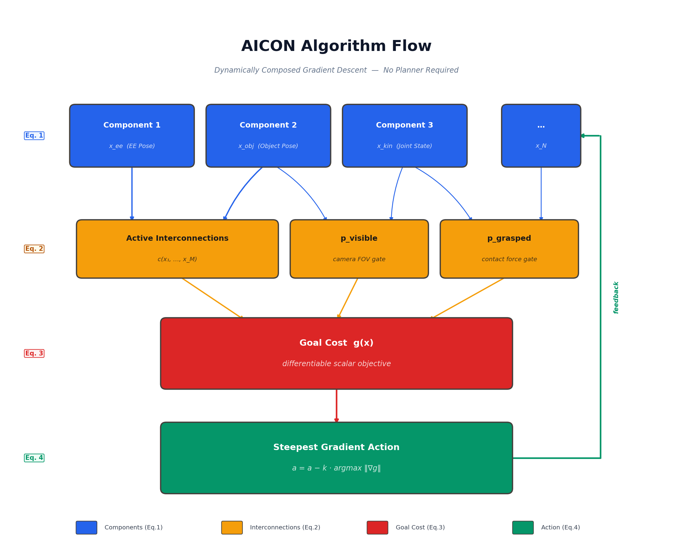
The entire algorithm is a loop:
- Components update their state estimates from sensor data (Eq. 1)
- Interconnections compute soft gates —
p_visible,p_grasped, etc. (Eq. 2) - Goal cost is differentiated through all paths in the graph (Eq. 3)
- The steepest gradient determines the next action (Eq. 4)
- The action changes the world → new sensor data → repeat
There is no planner, no policy, no search. The feedback arrow closes the loop. Let’s look at each piece.
Building Block 1: Components (Eq. 1)
Think of a “component” as a little module that tracks one thing about the world. The robot’s end-effector position. The estimated location of the drawer handle. Whether the gripper is open or closed.
Each component updates its estimate at every timestep:
x_t = f(x_{t-1}; c_1, c_2, ..., c_N)
“My new estimate depends on my old estimate plus whatever information is flowing in from other components.”
Here’s what this looks like in practice — an EKF tracking the drawer handle position (components.py):
class EKFComponent(BaseComponent):
    """Extended Kalman Filter — tracks one quantity with uncertainty."""

    def update(self, priors):
        # Predict step
        x_pred, F = self._process_model(self._state, priors)
        Sigma_pred = F @ self._Sigma @ F.T + self._Q

        # Update step (if we have a measurement)
        if "measurement" in priors:
            z = priors["measurement"]
            z_pred, H = self._measurement_model(x_pred)
            S = H @ Sigma_pred @ H.T + self._R
            K = Sigma_pred @ H.T @ torch.linalg.solve(S, torch.eye(...))
            self._state = x_pred + K @ (z - z_pred)
            self._Sigma = (I - K @ H) @ Sigma_pred
        else:
            self._state = x_pred
            self._Sigma = Sigma_pred
Everything is PyTorch, so gradients flow through torch.autograd. Not just an estimator — a differentiable estimator.
Building Block 2: Active Interconnections (Eq. 2)
Components share information through differentiable gates that turn on or off depending on the current state:
c(x_1, x_2, ..., x_M) — coupling changes based on state
Consider a visibility gate. Whether the wrist camera can see the drawer handle depends on where the end-effector is pointing. So p_visible is a soft sigmoid (interconnections.py):
class VisibilityGate(BaseInterconnection):
    def forward(self, ee_pose, object_pose):
        direction = object_pose[:3] - ee_pose[:3]
        cos_angle = F.cosine_similarity(direction, camera_forward, dim=0)
        return torch.sigmoid(self._sharpness * (cos_angle - self._threshold))
And p_grasped uses force-torque sensor readings:
class GraspGate(BaseInterconnection):
    def forward(self, distance, grip_force, hand_closed):
        p_close = torch.sigmoid(-self._dist_sharpness * (distance - self._dist_thresh))
        p_force = torch.sigmoid(self._force_sharpness * (grip_force - self._force_thresh))
        p_hand  = torch.sigmoid(self._hand_sharpness * (hand_closed - 0.5))
        return p_close * p_force * p_hand
This is the key insight. When p_visible = 0, the gradient path through vision is blocked. The algorithm naturally concludes: “I can’t optimize the grasp yet. The steepest gradient tells me to move the camera first.” Subgoal ordering falls out of the math — nobody programmed it.
Building Block 3: Steepest Gradient Action Selection (Eqs. 3–4)
The goal is a differentiable scalar cost. For opening a drawer 20 cm:
g(q) = (q − 0.20)²
The gradient propagates backward through all interconnections and components via the chain rule. Because different gates are open or closed, you get multiple gradient paths — each representing a different possible sub-goal.
The rule: pick the steepest one (gradient_descent.py):
# Compute all gradient paths
gradients = [path.gradient(action) for path in self._paths]

# Select steepest (Eq. 4)
norms = torch.stack([g.norm() for g in gradients])
best_idx = int(torch.argmax(norms).item())
grad_star = gradients[best_idx]

# Gradient descent (Eq. 3)
action_new = action - k * grad_star
That’s the entire control loop. No planner. No policy network.
Why It Works: The Locked Door Example
A point mass needs to reach (10, 0), but a wall at x=5 is locked. A button at (2, 4) opens it. The complete AICON implementation (demo_2d_locked_door.py):
class PointMassAICON:
    def step(self, lr=0.15):
        pos = self.agent_pos
        goal_dist = torch.norm(pos - self.goal_pos)
        dist_to_button = torch.norm(pos - self.button_pos)

        p_button_soft = torch.exp(-0.25 * (dist_to_button ** 2))
        door_current = door_prev + p_button * (1.0 - door_prev)

        factor = 1.0 + 10.0 * (1.0 - door_current)
        cost = goal_dist * factor + barrier * (1.0 - door_current)

        cost.backward()  # PyTorch does the rest
When the door is closed (door_current ≈ 0), factor = 11× — making the goal gradient weak relative to the button gradient. The agent:
- Moves toward the button (steepest gradient when door is closed)
- Touches the button (opens the door)
- Heads straight to the goal (steepest gradient when door is open)
No planner told it to do this.
python scripts/simple_demos/demo_2d_locked_door.pyScaling Up: Blocks World
AICON solves the classic Blocks World puzzle — rearranging block towers into a goal configuration — a benchmark that normally requires BFS or A*. The state is a matrix o[X,Y] (likelihood X is on Y) and vector c[X] (likelihood X is clear):
# Eq. 5: Is block X clear?
c[X] = 1 - (1/n) * sum(o[Y, X] for Y in blocks)

# Eq. 6: State update
o_new[X,Y] = o[X,Y] + c[X] * c[Y] * a_stack[X,Y] - c[X] * a_unstack[X,Y]
The gradient of the goal cost through these equations automatically decides whether to stack or unstack, and which blocks, and in what order (aicon_policy.py):
def _select_action(self, o, c, goal_cost):
    best_action, best_norm = ("stack", 0, 1), -1.0
    for X in range(n_blocks):
        for Y in range(n_blocks):
            if X == Y: continue
            if c[X] > 0.5 and c[Y] > 0.5:        # ∇_stack (Eq. 7)
                o_new = (o + c[X] * c[Y] * a_stack).clamp(0, 1)
                grad_norm = abs(goal_cost - goal_cost_fn(o_new))
                if grad_norm > best_norm:
                    best_action = ("stack", X, Y); best_norm = grad_norm
            if o[X,Y] > 0.5 and c[X] > 0.5:      # ∇_unstack (Eq. 8)
                o_new = (o - c[X] * a_unstack).clamp(0, 1)
                grad_norm = abs(goal_cost - goal_cost_fn(o_new))
                if grad_norm > best_norm:
                    best_action = ("unstack", X, Y); best_norm = grad_norm
    return best_action
Result: 100% solve rate on 130 randomly generated instances with 10–30 blocks, including tasks requiring 35+ steps. Matches optimal BFS in step count. No forward search.
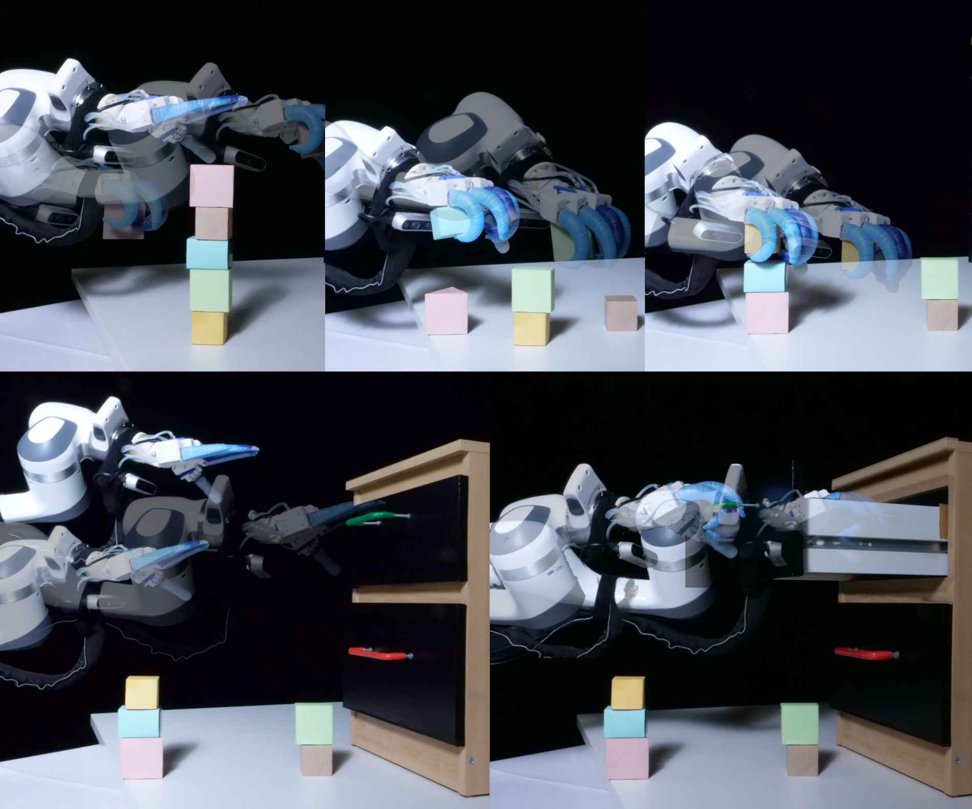
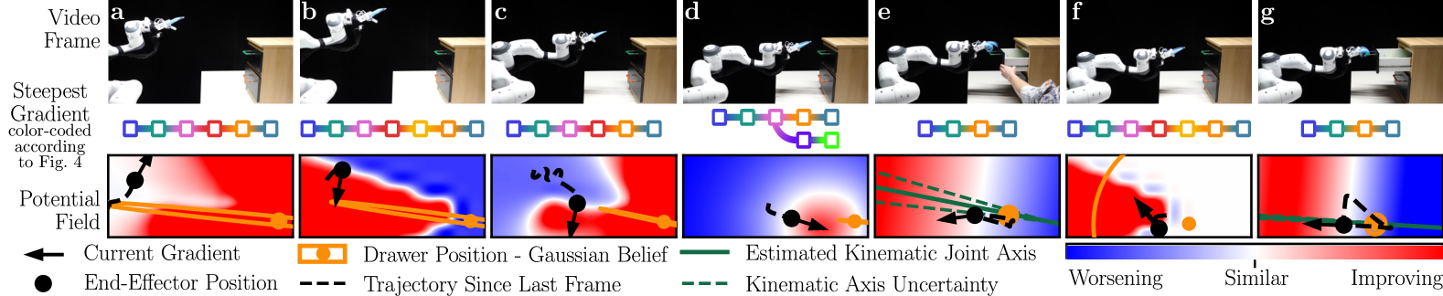
python scripts/run_blocks_world.pyReal-World: Drawer Manipulation
A Franka Panda with a wrist camera and force-torque sensor opens a physical drawer under uncertainty. Four components, two interconnections:
| Component | Tracks | Estimator |
|---|---|---|
| x_ee | End-effector pose | Direct kinematics |
| x_hand | Gripper state | Moving average |
| x_drawer | Handle position | EKF (covariance Σ) |
| x_kin | Joint params | EKF (covariance Σ) |
When Σ_drawer is large (high uncertainty), the steepest gradient path goes through reducing uncertainty — “move the camera to look around.” Once Σ_drawer shrinks, the gradient shifts to “reach and grasp.” After p_grasped flips to 1, it becomes “pull.” The robot sequences the entire task from one cost function: g(q) = (q − 0.20)².
Results vs. Planning Baselines
70 real-world trials: 7 conditions × 10 runs each. Baselines: state-space planner (fixed trajectory) and 67-dimensional belief-space planner (3 viewpoints + 2 kinematic explorations).
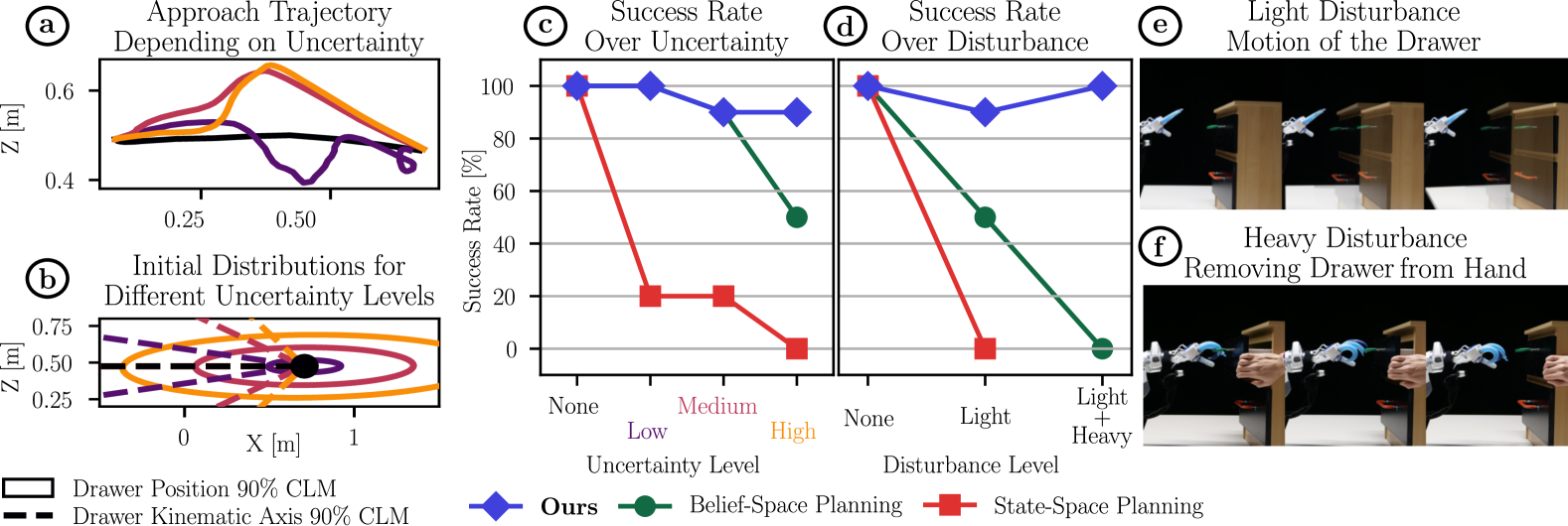
AICON handles both because it has no plan to become stale — the gradients recompute from live sensor feedback at every step. Under high uncertainty, it spontaneously invents triangulation — nobody programmed that behavior.
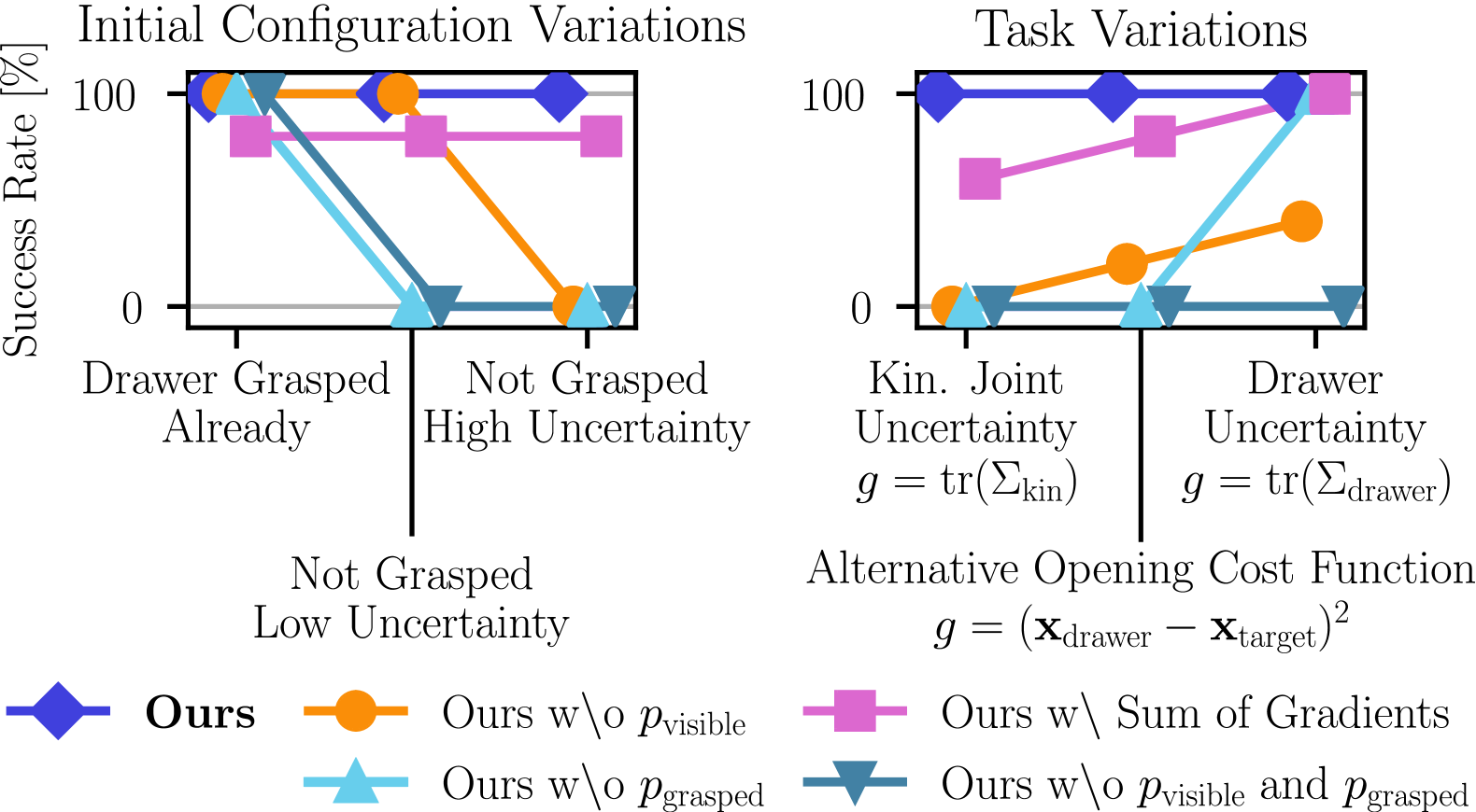
Ablations: Why the Gates Matter
Remove p_visible or p_grasped and performance craters. Sum all gradients instead of selecting the steepest and you get jerky, unstable motion. The steepest-gradient selector is crucial because competing subgoal gradients point in opposite directions and canceling them produces garbage.
My Take
What’s genuinely impressive:
- The math is minimal (sigmoid gates + chain rule + argmax) but the emergent behavior is sophisticated
- Zero-shot: no training, no reward shaping, no demonstrations
- Disturbance recovery is automatic — there’s no plan to invalidate, just gradients to recompute
- Matching BFS optimality in Blocks World with pure gradient descent is a striking result
Honest limitations:
- The graph structure is hand-designed per task. You need domain knowledge to pick the right components and gates
- Gradient path enumeration scales poorly. The drawer has ~12 paths; a kitchen scene would have thousands
- Everything must be differentiable. If your sensor model isn’t a PyTorch function, you’re stuck
Why it matters for this class:
Most current robotic AI either learns a policy end-to-end (which requires massive data) or uses a classical planner (which requires a precise world model). This paper suggests a third path: if you can express your world model differentiably, gradient descent handles task sequencing for free. That’s a structurally important insight, even if the current framework is limited to structured domains.
Code
Pure PyTorch, no simulator required for the demos:
git clone https://github.com/poad42/no_plan_everything_control
cd no_plan_everything_control

# Locked door (2D, instant, matplotlib)
python scripts/simple_demos/demo_2d_locked_door.py

# Blocks World solver
python scripts/run_blocks_world.py
Paper: arXiv:2503.01732
Supplementary videos: tu.berlin/robotics/papers/noplan